Legacy methods for rejecting artifacts in continuous and epoched data
This other section of the tutorial contains methods that are currently recommended for rejecting artifacts.
The current section refers to obsolete methods that are no longer recommended for artifact rejections, given better methods are now available. In EEGLAB 2019.1 and later version, make sure to select the option Show all menus from previous versions of EEGLAB in EEGLAB menu item File > Preference to be able to use the tools on this page.
Strategy: The approach used in EEGLAB for artifact rejection uses ‘statistical’ thresholding to ‘suggest’ epochs to reject from the analysis. Current computers are fast enough to allow easy confirmation and adjustment of suggested rejections by visual inspection, which our eegplot.m tool makes convenient. We therefore favor semi-automated rejection coupled with a visual inspection, as detailed below.
In practice, we favor applying EEGLAB rejection methods to independent components of the data, using a seven-stage method outlined below.
Examples: In all this section, we illustrate EEGLAB methods for artifact rejection using the same sample EEG dataset we used in the single-subject data analysis tutorial. These data are not perfectly suited for illustrating artifact rejection since they have relatively few artifacts! Nevertheless, by setting low thresholds for artifact detection, it is possible to find and mark outlier trials. Though these may not necessarily be artifact related, we use them here to illustrate how the EEGLAB data rejection functions work. We encourage users to make their own determinations as to which data to reject and to analyze using the set of EEGLAB rejection tools.
Rejecting artifacts in continuous data
Rejecting data channels based on channel statistics
Channel statistics may help determine whether to remove a channel or not. To compute and plot one channel statistical characteristics, use menu Plot → Data statistics → channel statistics. In the pop-up window below, enter the channel number. The parameter “Trim percentage” (default is 5%) is used for computing the trimmed statistics (recomputing statistics after removing tails of the distribution). If P is this percentage, then data values below the P percentile and above the 1-P percentile are excluded for computing trimmed statistics.
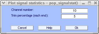
Pressing Ok will open the image below.
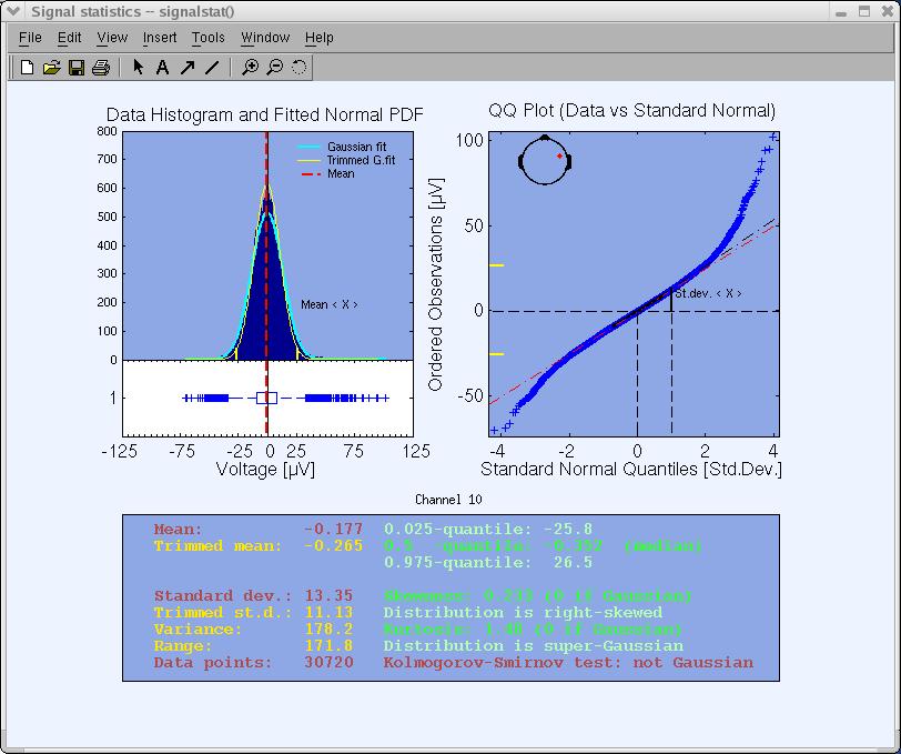
Some estimated variables of the statistics are printed as text in the lower panel to facilitate graphical analysis and interpretation. These variables are the signal mean, standard deviation, skewness, and kurtosis (technically called the four first cumulants of the distribution) and the median. The last text output displays the Kolmogorov-Smirnov test result (estimating whether the data distribution is Gaussian or not) at a significance level of p=0.05.
The upper left panel shows the data histogram (blue bars), a vertical red line indicating the data mean, a fitted normal distribution (light blue curve), and a normal distribution fitted to the trimmed data (yellow curve). The P and 1-P percentile points are marked with yellow ticks on the X axis. A horizontal notched-box plot with whiskers is drawn below the histogram. The box has lines at the lower quartile (25th-percentile), median, and upper quartile (75th-percentile) values. The whiskers are lines extending from each end of the box to show the extent of the rest of the data. The whisker extends to the most extreme data value within 1.5 times the width of the box. Outliers (‘+’) are data with values beyond the ends of the whiskers.
The upper right panel shows the empirical quantile-quantile plot (QQ-plot). Plotted are the quantiles of the data versus the quantiles of a Standard Normal (i.e., Gaussian) distribution. The QQ-plot visually helps to determine whether the data sample is drawn from a Normal distribution. If the data samples do come from a Normal distribution (same shape), even if the distribution is shifted and re-scaled from the standard normal distribution (different location and scale parameters), the plot will be linear.
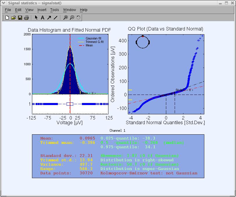
Empirically, ‘bad’ channels have distributions of potential values that are further away from a Gaussian distribution than other scalp channels. For example, plotting the statistics of periocular (eye) Channel 1 below, we can see that it is further away from a normal distribution than Channel 10 above. (However, Channel 1 should not itself be considered a ‘bad’ channel since ICA can extract the eye movement artifacts from it, making the remained data from this channel usable for further analysis of neural EEG sources that project to the face). The function plotting data statistics may provide an objective measure for removing a data channel.
Select menu item Edit → Select data to remove one or more data channels.
It is also possible to plot event statistics from the EEGLAB menu – see the EEGLAB event tutorial for details.
Note that the function above may also be used to detect bad channels in non-continuous (epoched) data.
Rejecting artifacts in epoched data
In contrast to continuous EEG data, we have developed several functions to find and mark for rejection of those data epochs that appear to contain artifacts using their statistical distributions. Since we want to work with epoched dataset, you should either load an earlier saved epoched dataset or, using the downloaded dataset (better loaded with channel locations info), use the following MATLAB script code:
EEG = pop_eegfilt( EEG, 1, 0, [], [0]); % Highpass filter cutoff freq. 1Hz.
[ALLEEG EEG CURRENTSET] = pop_newset(ALLEEG, EEG, CURRENTSET, 'setname', 'Continuous EEG Data'); % Save as new dataset.
EEG = pop_reref( EEG, [], 'refstate',0); % Re-reference the data
EEG = pop_epoch( EEG, { 'square' }, [-1 2], 'newname', 'Continuous EEG Data epochs', 'epochinfo', 'yes'); % Epoch dataset using 'square' events.
EEG = pop_rmbase( EEG, [-1000 0]); % remove baseline
[ALLEEG EEG CURRENTSET] = pop_newset(ALLEEG, EEG, CURRENTSET, 'setname', 'Continuous EEG Data epochs', 'overwrite', 'on');
% save dataset

[ALLEEG EEG] = eeg_store(ALLEEG, EEG, CURRENTSET); % store dataset
eeglab redraw % redraw eeglab to show the new epoched dataset
After having an epoched dataset, call the main window for epoched data rejection, select Tools → Reject data epochs → Reject data (all methods). The window below will pop up. We will describe the fields of this window in top-to-bottom order. First, change the bottom multiple-choice button reading Show all trials marked for rejection by the measure selected above or checked below to the first option: Show only the new trials marked for rejection by the measure selected above. We will come back to the default option at the end.

Rejecting epochs by visual inspection
As with continuous data, it is possible to use EEGLAB to reject epoched data simply by visual inspection. To do so, press the Scroll data button on the top of the interactive window. A scrolling window will pop up. Change the scale to ‘79’. Epochs are shown delimited by blue dashed lines and can be selected/deselected for rejection simply by clicking on them. Rejecting parts of an epoch is not possible.

Rejecting extreme values
During ‘threshold rejection’, the user sets up bounding values the data should not exceed. If the data (at the selected electrodes) exceeds the given limits during a trial, the trial is marked for rejection. Enter the following values under find abnormal values (which calls the pop_eegthresh.m function), and press CALC/PLOT. The parameters entered below tell EEGLAB that EEG values should not exceed +/-75 µV in any of the 32 channels (1:32 ) at any time within the epoch (‘‘-1000 ‘‘to 2000 ms).

Marked trials are highlighted in the eegplot.m window
(below) that then pops up. Now epochs marked for rejection may be un-marked manually simply by clicking on them. Note that the activity at some electrodes is shown in red, indicating the electrodes in which the outlier values were found. Press Update Marks to confirm the epoch markings.

At this point, a warning will pop up, indicating that the marked epochs have not yet been rejected and are simply marked for rejection. When seeing this warning, press Ok to return to the main rejection window.

Also, note that several thresholds may be entered along with separate applicable time windows. In the following case, in addition to the preceding rejection, additional epochs in which EEG potentials went above 25 µV or below -25 µV during the -500 to ms interval will be marked for rejection.
Rejecting abnormal trends
Artifactual currents may cause linear drift to occur at some electrodes. To detect such drifts, we designed a function that fits the data to a straight line and marks the trial for rejection if the slope exceeds a given threshold. The slope is expressed in microvolt over the whole epoch (50, for instance, would correspond to an epoch in which the straight-line fit value might be 0 µv at the beginning of the trial and 50 µ v at the end). The minimal fit between the EEG data and a line of minimal slope is determined using a standard R-square measure. To test this, in the main rejection window, enter the following data under findabnormal trends (which calls function pop_rejtrend.m), and press CALC/PLOT.
The following window will pop up. Note that the values we entered are clearly too low (otherwise, we could not detect any linear drifts in this clean EEG dataset). Electrodes triggering the rejection are again indicated in red. To deselect epochs for rejection, click on them. To close the scrolling window, press the Update marks button.

Note: Calling function pop_rejtrend.m either directly from the command line, or by selecting Tools > Reject data epochs > Reject flat line data, allows specifying additional parameters.
Rejecting improbable data
By determining the probability distribution of values across the data epochs, one can compute the probability of occurrence of each trial. Trials containing artifacts are (hopefully) improbable events and thus may be detected using a function that measures the probability of occurrence of trials. Here, thresholds are expressed in terms of standard deviations of the mean probability distribution. Note that the probability measure is applied both to single electrodes and the collection of all electrodes. In the main rejection window, enter the following parameters under find improbable data press Calculate (which calls function pop_jointprob.m), and then press PLOT.

The first time this function is run on a dataset, its computation may take some time. However, the trial probability distributions will be stored for future calls. The following display shows the probability measure value for every trial and electrode (each number at the bottom shows an electrode, and the blue traces indicate the trial values). On the right, the panel containing the green lines shows the probability measure over all the electrodes. Rejection is carried out using both single- and all-channel thresholds. To disable one of these, simply raise its limit (e.g., to 15 std.). The probability limits may be changed in the window below (for example, to 3 standard deviations). The horizontal red lines shift as limit values are then modified. Note that if you change the threshold in the window below, the edit boxes in the main window will be automatically updated (after pressing the UPDATE button).

It is also possible to look in detail at the trial probability measure for each electrode by clicking on its sub-axis plot in the above window. For instance, by clicking on electrode number two on the plot, the following window would pop up (from left to right, the first plot is the ERPimage) of the square values of EEG data for each trial, the second plot indicates which trials were labeled for rejection (all electrodes combined), and the last plot is the original probability measure plot for this electrode with limits indicated in red).

Close this window and press the UPDATE button in the probability plot window to add to the list of trials marked for rejection.
Now press the ‘Scroll data button to obtain the standard scrolling data window. Inspect the trials marked for rejection, make any adjustments manually, then close the window by pressing UPDATE MARKS.

Rejecting abnormally distributed data
Artifactual data epochs sometimes have very ‘peaky’ activity value distributions. For instance, if a discontinuity occurs in the activity of data epoch for a given electrode, the activity will be either close to one value or the other. To detect these distributions, a statistical measure called kurtosis is useful. Kurtosis is also known as the fourth cumulant of the distribution (the skewness, variance, and mean being the first three). A high positive kurtosis value indicates an abnormally ‘peaky’ distribution of activity in a data epoch, while a high negative kurtosis value indicates abnormally flat activity distribution. Once more, single- and all-channel thresholds are defined in terms of standard deviations from mean kurtosis value. For example, enter the following parameters under ‘‘find abnormal distribution ‘’ press Calculate (which calls function pop_rejkurt.m), then press PLOT.

In the main rejection window, note that the Currently marked trials field have changed to 5. In the plot figure, all trials above the threshold (red line) are marked for rejection. Note that there are more than 5 such lines. The figure presents all channels, and the same trial can exceed the threshold several times in different channels, and therefore there are more lines than marked trials.

As with probability rejection, these limits may be updated in the pop-up window below, and pressing Scroll data in the main rejection window (above) brings up the standard data scrolling window display which may be used to manually adjust the list of epochs marked for rejection.
Rejecting abnormal spectra
According to our analysis, rejecting data epochs using spectral estimates may be the most effective method for selecting data epochs to reject for analysis. In this case, thresholds are expressed in terms of amplitude changes relative to baseline in dB. To specify that the spectrum should not deviate from baseline by +/-50 dB in the ‘’ 0-2’’ Hz frequency window, enter the following parameters under ‘’ find abnormal spectra’’ (which calls the pop_rejspec.m function), then press CALC/PLOT.

Computing the data spectrum for every data epoch and channel may take a while. We use a frequency decomposition based on the Slepian multitaper (MATLAB pmtm function) to obtain more accurate spectra than using standard Fourier transforms. After computing the trial spectra, the function removes the average power spectrum from each trial spectrum and tests whether the remaining spectral differences exceed the selected thresholds. Here, two windows pop up (as below), the top window being slaved to the bottom. The top window shows the data epochs, and the bottom window the power spectra of the same epochs. When scrolling through the trial spectra, the user may use the top window to check what caused a data trial to be labeled as a spectral outlier. After further updating the list of marked trials, close both windows by pressing UPDATE MARKS in the bottom window.


As with standard rejection of extreme values, several frequency thresholding windows may be defined. In the window below, we specify that the trial spectra should again not deviate from the mean by +/-50 dB in the 0-2 Hz frequency window (good for catching eye movements) and should not deviate by +25 or -100 dB in the 20-40 Hz frequency window (useful for detecting muscle activity).

Inspecting current versus previously proposed rejections
To compare the effects of two different rejection thresholds, the user can plot the currently and previously marked data epochs in different colors. To do this, change the option in the long rectangular tab under Plotting options (at the bottom of the figure). Select Show previous and new trials marked for rejection by this measure selected above. For instance, using ‘’ abnormal distribution’’, enter the following parameters, and press Scroll data.

The scrolling window appears and now shows that at trials 11 & 12, the blue window is actually divided into two, with dark blue on the top and light blue on the bottom. Dark blue indicates that the trial is currently marked as rejected. The light blue indicates that the trial was already rejected using the previous rejection threshold.

Note: Pressing UPDATE MARKS updates the currently rejected trials and optional visual adjustments. Previously rejected trials are ignored and can not be removed manually in the plot window.
Inspecting results of all rejection measures
To visually inspect data epochs marked for rejection by different rejection measures, select Show all trials marked for rejection measures by the measure selected above or checked below in the long rectangular tab under ‘’ Plotting options’’. Then press CALC/PLOT under Find abnormal spectra. Rejected windows are divided into several colored patches, each color corresponding to a specific rejection measure. Channels colored red are those marked for rejection by any method.

When visually modifying the set of trials labeled for rejection in the window above, all the current rejection measures are affected and are reflected in the main rejection window after you press the UPDATE MARKS button.
Notes and strategy
- The approach we take to artifact rejection is to use statistical thresholding to suggest epochs to reject from the analysis. Current computers are fast enough to allow easy confirmation and adjustment of suggested rejections by visual inspection. Therefore, we favor semi-automated rejection coupled with a visual inspection.
- All the functions presented here can also be called individually through Plot -> Reject data epochs or from the MATLAB command line.
- After labeling trials for rejection, it is advisable to save the dataset before actually rejecting the marked trials (marks will be saved along with the dataset). This gives one the ability to go back to the original dataset and recall which trials were rejected.
- To actually reject the marked trials, either use the option Reject marked trials at the bottom of the main rejection window, or use the main EEGLAB window options Tools > Reject data epochs > Reject marked epochs.
- All these rejection measures are useful, but if one does not know how to use them, they may be inefficient. Because of this, we have not provided standard rejection thresholds for all the measures. In the future we may include such information in this tutorial. The user should begin by visually rejecting epochs from some test data, then adjust parameters for one or more of the rejection measures, comparing the visually selected epochs with the results of the rejection measure. All the measures can capture both simulated and real data artifacts. In our experience, the most efficient measures seem to be the frequency threshold and linear trend detection.
- We typically apply semi-automated rejection to the independent component activations instead of to the raw channel data, as described below.
Rejection based on independent data components
Rejecting data based on ICA component activity
To reject data by visual inspection of its ICA component activations, select Plot → Component activation (scroll) (calling pop_eegplot.m. It is often easier to spot artifacts in ICA component activation than it is in raw data. Rejecting portions of data will reject it for both EEG data and ICA components.
Note that marked epochs can be kept in memory before being actually rejected - if the option Reject marked trials (checked=yes) below is not set. Thus it is possible to mark trials for rejection and then to come back and update the marked trials. The first option - Add to previously marked rejections (checked=yes) - allows us to include previous trial markings in the scrolling data window or to ignore/discard them.
Since it is the first time we have used this function on this dataset, the option to plot previously marked trials won’t have any effect.
Check the checkbox to reject marked trials, so that the marked trials will be immediately rejected when the scrolling window is closed. Press Ok.
First, adjust the scale by entering 10 in the scale text edit box (lower right).
Now, click on the data epochs you want to mark for rejection. For this exercise, highlight two epochs.
You can then deselect the rejected epochs by clicking again on them.
Press the Reject button when finished and enter a name for the new dataset (the same dataset minus the rejected epochs), or press the Cancel button to cancel the operation.
At this point, you may spend some time trying out the advanced rejection functions we developed to select and mark artifactual epochs based on ICA component maps and activations.
Then, after rejecting ‘bad’ epochs, run ICA decomposition again. Hopefully, by doing this, you may obtain a ‘cleaner’ decomposition.
Semi-automated artifact rejection
We usually apply the measures described in the previous sections to the activations of the independent components of the data. As independent components tend to concentrate artifacts, we have found that bad epochs can be more easily detected using independent component activities. The functions described above work exactly the same when applied to data components as when they are applied to the raw channel data. Select Tools > Reject data using ICA > Reject data (all methods). We suggest that the analysis be done iteratively in the following seven steps:
- Visually reject unsuitable (e.g., paroxysmal) portions of the continuous data.
- Separate the data into suitable short data epochs.
- Perform ICA on these epochs to derive their independent components.
- Perform semi-automated and visual-inspection based rejection of data epochs on the derived components. (*)
- Visually inspect and select data epochs for rejection.
- Reject the selected data epochs.
- Perform ICA a second time on the pruned collection of short data epochs – This may improve the quality of the ICA decomposition, revealing more independent components accounting for neural, as opposed to mixed artifactual activity. If desired, the ICA unmixing and sphere matrices may then be applied to (longer) data epochs from the same continuous data. Longer data epochs are useful for time/frequency analysis and may be desirable for tracking other slow dynamic features.
- Inspect and reject the components. Note that components should NOT be rejected before the second ICA, but after.
(*) After closing the main ICA rejection window, select Tools → Reject data using ICA → Export marks to data rejection, and then Tools → Reject data epochs → Reject by inspection to visualize data epochs marked for rejection using ICA component activities.