Study Statistics and Visualization Options
Statistics are at the core of EEG analysis. Here, we will briefly review how to use different types of statistics at the group level. For an introduction to robust statistics in EEGLAB, read the statistics theory section of the tutorial or watch the series of short videos below. Click on the icon on the top right corner to access the list of videos in the playlist.
Table of contents
Channel ERP statistics
EEGLAB allows users to use either parametric or non-parametric statistics to compute and estimate the reliability of these differences within STUDY designs. Below we illustrate the use of these options on scalp channel ERPs, though they apply to all measures and are valid for both scalp channels and independent component (or other) source activity clusters.
Load tutorial data and precompute ERPs
For this tutorial we will use the STERN STUDY (0.9 Gb). Please download the data on your computer. See the STUDY design section of the tutorial for more information about this dataset.
Use menu item File → Load existing study and select the stern_3designs.study file. After loading the data, to review the STUDY design, use the Study → Select/Edit study design menu item. See the STUDY design tutorial for details on how to create these designs.
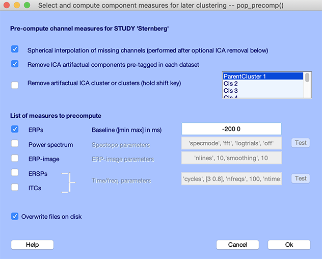
Before plotting the channel measures, you must precompute them using the Study → Precompute channel measures menu item, as shown below.
- Select the checkbox Remove ICA artifactual components pre-tagged in each dataset
- Select the ERPs checkbox
- Change the baseline to -200 to 0 as shown below
- Press Ok
1-way ANOVA on ERP plots
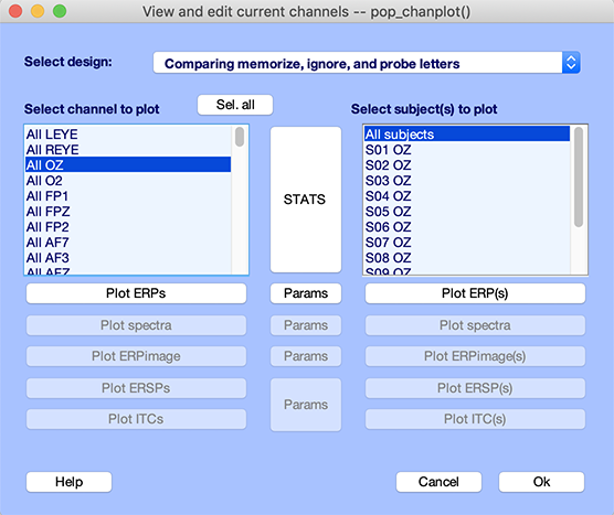
Select menu item Study → Plot channel measures. Select channel Oz in the left column, as shown below.
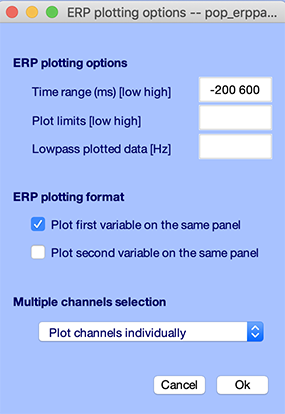
First, select a shorter time range for plotting ERPs. Press the Params button and enter a time range from -200 ms to 600 ms as shown below. Select the checkbox for plotting the first independent variable values (i.e., conditions) on the same panel. Press Ok.
In the middle of the two lists of channels, click on the large STATS pushbutton. The following graphic interface pops up.
- Click on the Compute 1st independent variable statistics checkbox. Note that, since there were no second independent variable selected in this study design, the Compute 2nd independent variable statistics is not be available.
- Select Use permutation statistics in the dropdown list for the type of statistics instead of Parametric statistics. While parametric statistics might be adequate for exploring your data, it is better to use permutation-based statistics to plot final results.
- Select the False Discovery Rate (FDR) method in the dropdown list to correct for multiple comparisons.
- Enter 0.05 for the p-value threshold.
- Press Ok.

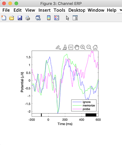
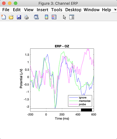
Then press the Plot ERPs button on the right column. The following plot pops up, showing the ERPs for the three types of letter ignore, memorize, and probe. We observe a significant difference from about 450 ms to about 570 ms, indicated by the black bar under the ERP plots. We also observe transient significance in the baseline at about -100 ms.
Let’s try a different method to correct for multiple comparisons. Click on the STATS button again:
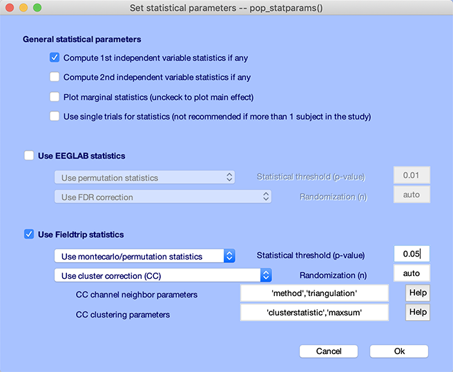
- Check the checkbox Use FieldTrip statistics.
- Select montecarlo/permutation as the type of statistics.
- Select Use cluster correction (CC) to correct for multiple comparisons. Refer to the FieldTrip documentation to tune the parameters for the cluster correction (use the defaults for now).
- Use 0.05 for the statistics threshold.
- Press Ok.
Then press the Plot ERPs button again on the left column. The region of significance is similar to the previous FDR correction for multiple comparisons method, although the transient statistical difference in the baseline has disappeared.
1-way ANOVA on ERP scalp topographies
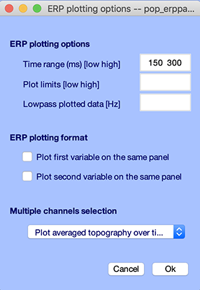
Now let’s perform statistics on scalp topographies. Press again the Params button, and select the 150 to 300 ms time range. Select Plot averaged topography over time in the bottom panel and press Ok.
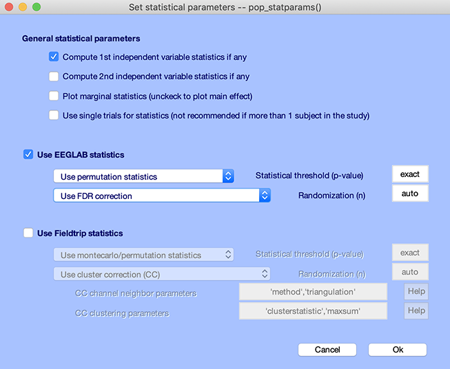
Press the STATS button and select permutation statistics with FDR correction for multiple comparisons as shown below.
Now press the Sel all. button in the right column to select all channels. Then press the Plot ERPs button. The following plot pops up. This plot shows scalp topographies from 150 ms to 300 ms for the different conditions, and the associated p-value map (extreme right). The difference, in this case, seems driven by the probe condition. In the following section, we will look at the difference between the ignore and memorize letters.

2-way ANOVA
Let’s select the third design in the STUDY plotting interface as shown below (dropdown list in the upper part of the GUI). This design compares the ignore and memorize conditions under different memory loads (from 0 to 5). The STUDY design section of the tutorial describes how this design was created. Select also the Oz channel.
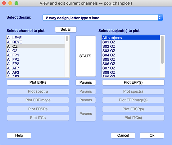
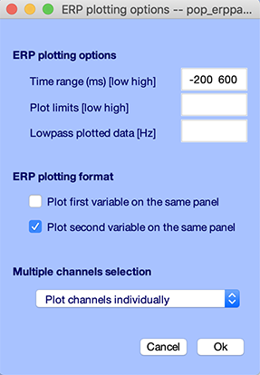
Now press the Params button and change the plotting time range to -200 ms to 600 ms as shown below. Check the checkbox to Plot section variable on the same panel. Make also sure to select the option to Plot channels individually. Press Ok.
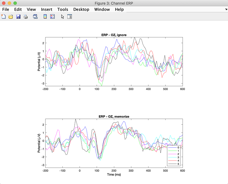
Press Plot ERPs button. The plot below pops up.
We will study statistics of scalp topographies in the 150 ms to 300 ms range. To do so, press the Params button and enter a time range from 150 ms to 300 ms as shown below. Make also sure to select the option to Plot averaged topography over time. You may or may not uncheck the checkbox to Plot section variable on the same panel (this has no consequences since scalp topographies for different conditions cannot be plotted on the same panel). Press Ok.

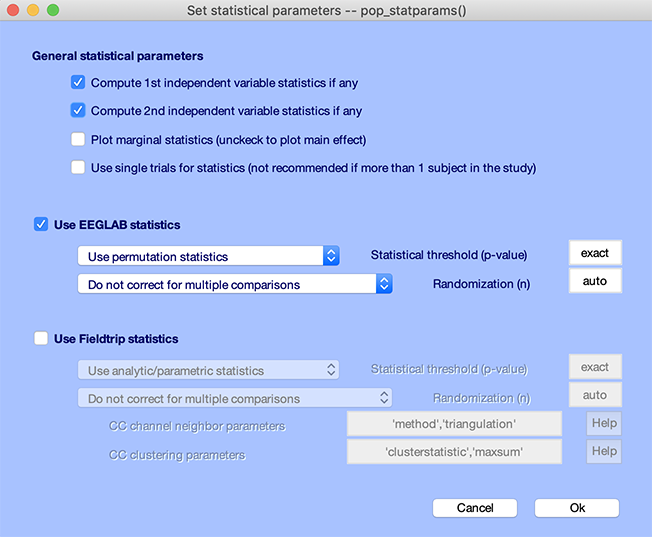
Press the STATS button and select both independent variables as shown below. Select permutation statistics with no correction for multiple comparisons. Press Ok.
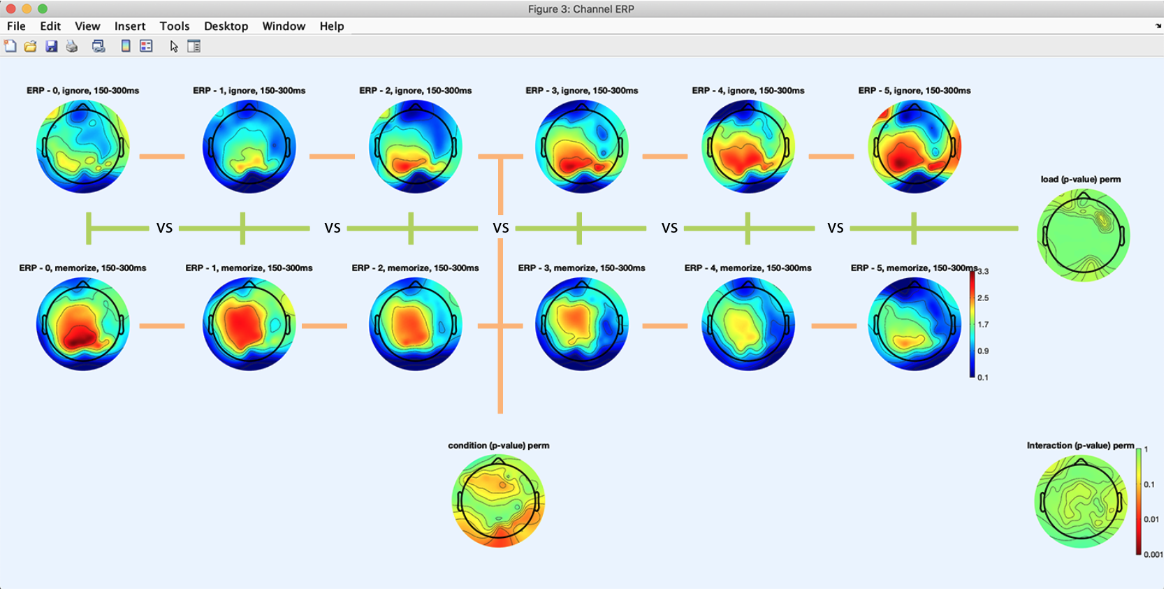
Press the Plot ERPs button again. The following plot pops up and shows an array of 2 x 5 scalp topographies for the 2 x 5 design (2 conditions ignore and memorize times 5 memory loads). The scalp topography on the bottom shows the p-value map across conditions (ignore vs. memorize). The scalp topography on the right shows the p-value map across memory loads. The scalp topography in the bottom right corner shows the p-value for the ANOVA interaction term between conditions and memory loads. We observe a statistical trend for the memory load, meaning that memory load may lead to different scalp topographies in the time range of interest. Note that we added the green and orange lines with photoshop to help illustrate how the main effect for each variable is calculated. The load variable statistics is an ANOVA across 7 different loads. By contrast, the condition variable compares two conditions.
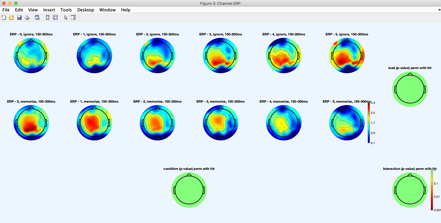
We now select the STATS button again and add check the FDR correction for multiple comparisons checkbox (not shown). Press the Plot ERPs button again. As shown below, the p-value statistical maps are all green indicating no significant effect.
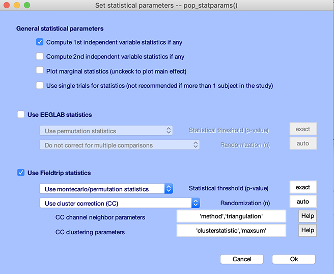
Let’s try the cluster method to correct for multiple comparisons. Press the STATS button again. Check the checkbox to compute statistics only on the first variable (FieldTrip cannot perform 2-way ANOVAs, only 1-way ANOVAs) and check the checkbox Use FieldTrip statistics. Select Montecarlo/permutation as the type of statistics and Use cluster correction (CC) method to correct for multiple comparisons. Press Ok.
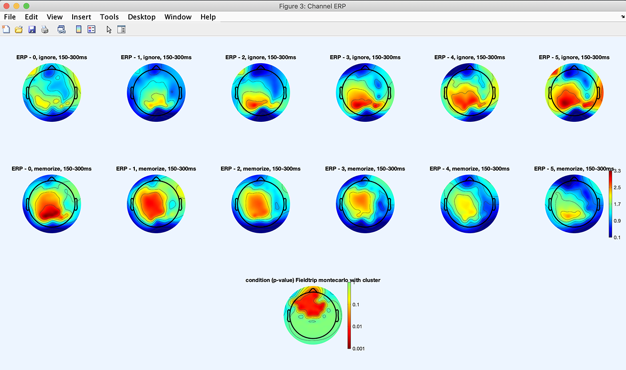
Press the Plot ERPs button, and the following plot appears, showing a statisticallly significant difference between the ignore and memorize conditions.
To look at the marginal statistics, select the STATS button and check the checkbox to compute marginal statistics (only the upper panel of the GUI is shown below).

Then press the Plot ERPs button again. We see that the statistical difference observed previously is mostly due to memory loads 0, 1, and 2.
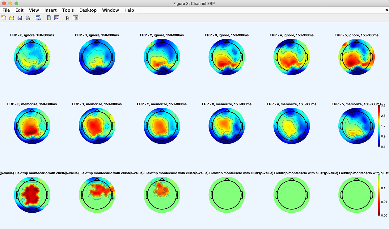
Note that the analysis above is preliminary at best. The fact that uncorrected significance was low for the comparison between conditions, then showed up as significant with the cluster analysis, indicate weakly significant regions. Based on the scalp topography for the cluster analysis, it is unclear if significance is below 0.05. You may retrieve the p-values from the command line, as explained in the group analysis scripting tutorial.
In general, we advise focusing on reporting unambiguous results (significance below 0.005 after correction for multiple comparisons).
Statistics on spectra, ITC, and ERSP
The graphic interfaces for both power spectral and ERSP/ITC measures are similar to those used for ERPs and need not be described in detail. Statistics options, selected in the statistics graphic interface (STATS button), apply to all measures. You may refer to the relevant function help messages for more detail.
ICA component cluster statistics
The same methods for statistical comparison apply to both groups of data channels and component clusters.
The plotting interface is virtually identical for channels and ICA component clusters. In the channel plotting interface, the left column is used to plot grand averages, and the right column to plot individual subjects. Similarly, for clusters, the left column plots ICA clusters, and the right column plot individual components.
General Linear Modelling using LIMO
For more complex statistical designs, one must use the LIMO plugin. The LIMO toolbox allows you to use general linear modeling approaches on an arbitrarilly large number of categorical and continuous variables. For more information, refer to the LIMO plugin documentation and the LIMO tutorial video series.
Single-subject statistics
When a STUDY only contains data from a single subject, you may also compute single-subject statistics. Below, we illustrate the process using ERPs, but we would use a similar procedure on other measures, including spectra, ERP-image, ERSP, and ITC.
In this section of the tutorial, we will use the 5-subject experiment (450Mb), although we will only use one of the five subjects. See the STUDY creation tutorial for more information on this data.
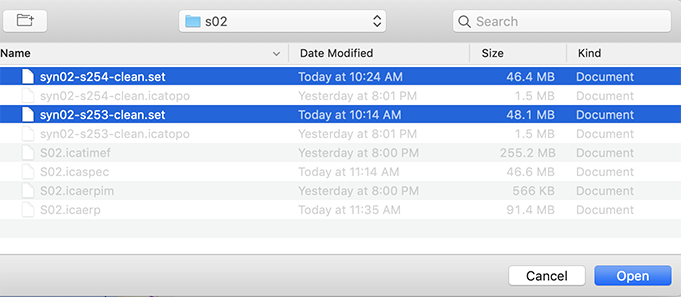
Restart EEGLAB. After uncompressing the data archive, load the two datasets for subject two (s02) using the File → Load existing dataset menu item. When several datasets are in the same folder, they may be selected and loaded in EEGLAB simultaneously, as shown below.
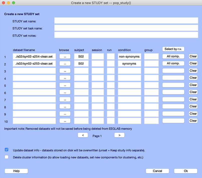
Then use the File → Create study → Using all loaded datasets menu item. The GUI below pops up. Press Ok.
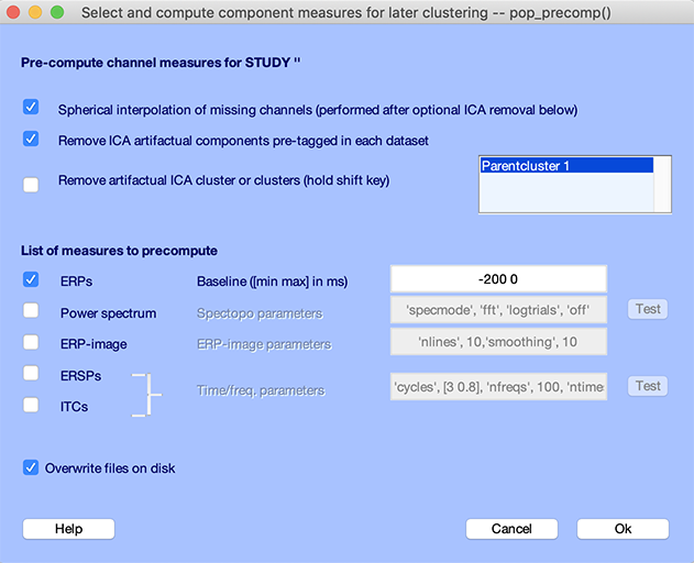
Select the Study → Precompute channel measures menu item. The GUI below pops up. Select the checkbox to Remove artifactual ICA components pre-tagged in each dataset. Select the ERPs checkbox and enter -200 ms to 0 ms for the baseline, as shown below. Press Ok.
Next, select the Study → Plot channel measures menu item. The GUI below appears. Select channel Oz in the right column.
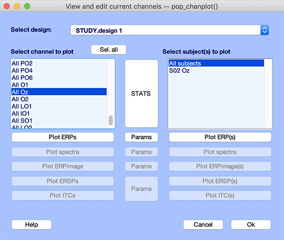
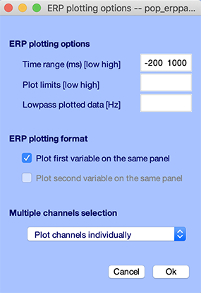
Now, press the Params button next to the Plot ERPs button. Enter -200 ms to 1000 ms for the time range. Check the checkbox Plot first variable on the same panel. Press Ok.
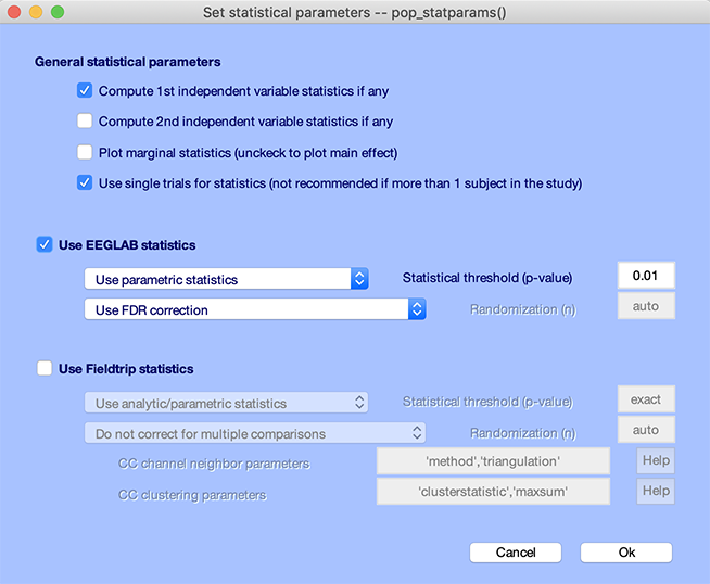
Press the STATS button. Check the checkboxes Compute 1st independent variable statistics if any and Use single trials for statistics. Select Use FDR correction for the correction for multiple comparisons method. Enter 0.01 for the p-value threshold, as shown below. Press Ok.
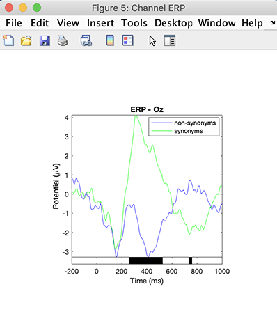
Now, click on the Plot ERPs button. The ERP for both conditions is shown with regions of significance indicated by black rectangles. We observe a typical N400 effect, with ERPs differing between the semantic conditions at about 400 ms after stimuli presentation.
The use of single trials is not restricted to single-subject statistics. When multiple subjects are present, trials may be pooled for all subjects. However, we do not recommend using this option for more than one subject because it alters the null hypothesis.
When performing statistics on a single subject, the null hypothesis pertains to the trials of this subject. When performing statistics on multiple subjects, the null hypothesis relates to the population of subjects. Using single-trials statistics with multiple subjects would mean that the null hypothesis pertains to the trials of the selected subjects (and not the population of subjects), which greatly limits the data interpretation.
The LIMO plugin also allows performing single-subject statistics in EEGLAB.