Introduction
Below a graphical explanation of the meaning of cutoff frequencies, pass band, stop band, as well as transition bands. 
In the default Windowed Sync filter, we have given some reasonable start values there for the filter order: 2 * cutoff freq for highpass and bandpass (for cutoff < 2Hz). 20 to 40% of cutoff freq for lowpass and 1 to 5 Hz for line noise bandstop. The basic rule is to have the transition band as wide (roll-off soft) as possible to avoid artifacts but separated from the signal of interest.
Filtering the data
To remove linear trends, it is often desirable to high-pass filter the data. High-pass filtering the data at 1 Hz is also recommended to obtain good quality ICA decompositions (Klug & Gramann, 2020). Low-pass filtering high-frequency noise is also sometimes necessary.
Load the sample EEGLAB dataset
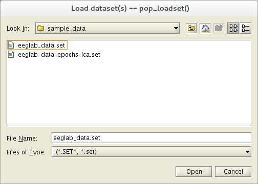
Select menu item File and press sub-menu item Load existing dataset. Select the tutorial file “eeglab_data.set” which is distributed with the toolbox, located in the “sample_data” folder of EEGLAB. Then press Open.

Removing linear trends
We recommend filtering continuous EEG data before epoching or artifact removal, although epoched data can also be filtered with this function (each epoch being filtered separately). Filtering the continuous data minimizes the introduction of filtering artifacts at epoch boundaries.
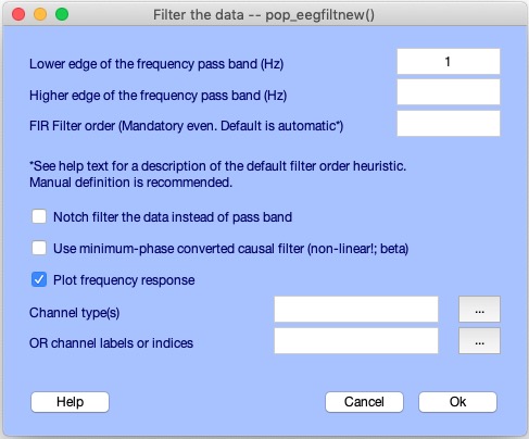
Select Tools → Filter the data → Basic FIR filter (new, default), enter 1 (Hz) as the Lower edge frequency, and press Ok.
Note that the EEGLAB legacy filter is no longer recommended but maintained for backward compatibility purposes only (Widmann & Schröger, 2012).

A window will pop up to ask for the name of the new dataset. We choose to modify the dataset name and to overwrite the parent dataset by checking the Overwrite parent checkbox, then pressing the Ok button.
Note that if high-pass and low-pass cutoff frequencies are BOTH selected, low-pass and high-pass parts will have the same slopes. Frequently, the low-pass slope is therefore steeper than necessary. To avoid this problem, we recommend first applying the low-pass filter and then, in a second call, the high-pass filter (or vice versa).
After you filter your data, check that the filter has been applied by selecting the Plot → Channel spectra and maps menu item to plot the data spectra. You might notice that filtered-out frequency regions might show ‘ripples’, unavoidable but hopefully acceptable filtering artifacts.
Note that removing data portions containing major artifacts (by visual inspection), such as large spikes in the data, before filtering can be preferable since filtering can “spread” the artifact out over “good” data, requiring more data to be rejected after filtering. When you remove major artifacts, a “boundary” event replaces the removed data. Filtering is only applied to continuous data segments, not across boundaries.
Filtering for connectivity analysis
High pass filtering introduces dependencies in neighboring data samples and is often not recommended for connectivity analysis. In this case, it is usually better to apply piecewise detrending to remove data trends. Piecewise detrending is available in the SIFT EEGLAB plugin, for example.
For causal analysis (assessing if one process causes another), call menu item Tools → Filter the data → Basic FIR filter (legacy) and check the checkbox Use causal filter. By default, the EEGLAB legacy filter applies the filter forward and then again backward to ensure that phase delays introduced by the filter are nullified. When using a causal filter, the filter is only applied forward, so phase delays might be introduced and not compensated for. However, causal relationships are preserved.
Filtering without the signal processing toolbox
If the MATLAB Signal Processing Toolbox is present, the EEGLAB legacy filter uses the MATLAB routine filtfilt.m. This applies the filter forward and then again backward to ensure that phase delays introduced by the filter are nullified.
If the MATLAB Signal Processing toolbox is not present, the EEGLAB legacy filter may use a simple filtering method involving the inverse Fourier transform. To do this, call the Tools → Filter the data → Basic FIR filter (legacy) menu item and check the checkbox Use (sharper) FFT linear filter instead of FIR filtering.
Non-linear infinite impulse response filter and other filters
A infinite impulse response (IIR) filter plugin is also distributed as a plugin to EEGLAB. Once the iirfilt plugin is installed, it can be accessed from the menu item Tools → Filter the data → Short IIR filter . This functionality uses the same graphical interface as the FIR filtering option described above. Although IIR filters usually introduce different phase delays at different frequencies, this is compensated for by applying filtering in reverse using MATLAB function filtfilt.m. Note that the order of infinite impulse response (IIR) filters cannot be directly compared to the order finite impulse response (FIR) filters due to recursive operation.
There is much more to be learned about filtering and more filtering options available in MATLAB itself. There is also no ideal filter for EEG data. For example, the impact of high-pass filters on ERP data is currently under discussion. In practice, we suggest you talk to your colleagues about the pros and cons of using different filter solutions. See also our Q/A filtering page including relevant references. For an introduction into definitions and concepts you may also check Widmann et al., 2015.
Alternative to filtering for line noise removal
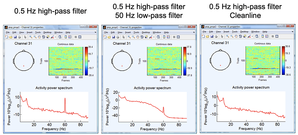
Another common use for bandpass filtering is to remove 50-Hz or 60-Hz line noise – also known as notch filtering. However, to remove line noise, one may also use the CleanLine EEGLAB plugin. This plugin adaptively estimates and removes sinusoidal (e.g., line) noise fusing multi-tapering and a Thompson F-statistic. Note that the version of CleanLine implemented in the PREP pipeline claims to have critical fixes PREP although this claim has not been verified yet. As shown in the comparison figure below, when this method works (and it does not always work), the result can be spectacular.
