Group-level analyses using EEGLAB scripts
Building a STUDY from the graphic interface (as described in previous sections) calls eponymous MATLAB functions that may also be called directly by users. Below we briefly describe these functions. See their MATLAB help messages for more information. Functions whose names begin with std_ take STUDY and/or EEG structures as arguments and perform signal processing and/or plotting directly on channel or cluster activities. Whenever relevant, feel free to look up documentation in the part of the tutorial describing the STUDY structure.
Table of contents
Creating a STUDY
If a STUDY contains many datasets, you might prefer to write a small script to build the STUDY instead of using the pop_study.m GUI. This is also helpful when you need to build many studies or to repeatedly add files to an existing STUDY.
Important note: If you want to modify the STUDY structures, you need to be careful as the STUDY checking function (std_checkset.m) performs multiple checks to keep it compatible with the datasets it represents. So this function might undo your changes (a warning will be issued on the command line). It is often possible to modify the datasets themselves to achieve the same goal, and changes will be automatically reported in the STUDY structures.
Below is a MATLAB script calling the GUI-equivalent command line function std_editset.m from the “5subjects” folder (you may download tutorial data here) then change the path to the folder you have uncompressed. The code snippets used on this page are available at study_script.m
[STUDY ALLEEG] = std_editset( STUDY, [], 'name','N400STUDY',...
        'task', 'Auditory task: Synonyms Vs. Non-synonyms, N400',...
        'filename', 'N400empty.study','filepath', './',...
        'commands', { ...
      { 'index' 1 'load' 'S02/syn02-S253-clean.set' 'subject' 'S02' 'condition' 'synonyms' }, ...
      { 'index' 2 'load' 'S05/syn05-S253-clean.set' 'subject' 'S05' 'condition' 'synonyms' }, ...
      { 'index' 3 'load' 'S07/syn07-S253-clean.set' 'subject' 'S07' 'condition' 'synonyms' }, ...
      { 'index' 4 'load' 'S08/syn08-S253-clean.set' 'subject' 'S08' 'condition' 'synonyms' }, ...
      { 'index' 5 'load' 'S10/syn10-S253-clean.set' 'subject' 'S10' 'condition' 'synonyms' }, ...
      { 'index' 6 'load' 'S02/syn02-S254-clean.set' 'subject' 'S02' 'condition' 'non-synonyms' }, ...
      { 'index' 7 'load' 'S05/syn05-S254-clean.set' 'subject' 'S05' 'condition' 'non-synonyms' }, ...
      { 'index' 8 'load' 'S07/syn07-S254-clean.set' 'subject' 'S07' 'condition' 'non-synonyms' }, ...
      { 'index' 9 'load' 'S08/syn08-S254-clean.set' 'subject' 'S08' 'condition' 'non-synonyms' }, ...
      { 'index' 10 'load' 'S10/syn10-S254-clean.set' 'subject' 'S10' 'condition' 'non-synonyms' }, ...
        { 'dipselect' 0.15 } });
Above, each line of the command loads a dataset.
The last line preselects components whose equivalent dipole models have less than 15% residual variance from the component scalp map. See >> help std_editset for more information.
Notice that the path to the datasets in the code above is a relative path. Then, to run the same code snippet, your current directory in MATLAB should contain the datasets.
Once you have created a new STUDY (or once you have loaded it from disk), both the STUDY structure and its corresponding ALLEEG array of resident EEG structures will be variables in the MATLAB workspace.
Typing >> STUDY on the MATLAB command line will list field values:
>> STUDY =

  struct with fields:

          history: 'STUDY = []; [STUDY ALLEEG] = std_checkset(STUDY, ALLEEG);'
          datasetinfo: [1×10 struct]
          name: 'N400STUDY'
          task: 'Auditory task: Synonyms Vs. Non-synonyms, N400'
          notes: ''
          filename: 'N400empty.study'
          filepath: '.'
          subject: {'S02'  'S05'  'S07'  'S08'  'S10'}
          group: {}
          session: []
          condition: {'non-synonyms'  'synonyms'}
          etc: [1×1 struct]
          cache: []
          preclust: [1×1 struct]
          cluster: [1×1 struct]
          changrp: [1×61 struct]
          design: [1×1 struct]
          currentdesign: 1
          saved: 'yes'
Because conditions have been defined in the individual datasets (synonyms and non-synonyms), EEGLAB will automatically create a STUDY design to compare these two conditions. You may also use the std_makedesign.m function from the command line to create different design. Try creating design in the EEGLAB graphic interface and look at what is returned in the history (via the eegh.m function). If you wish to add event information for creating designs, refer to the section of the tutorial for adding event information for group analysis.
Computing and plotting channel measures
Computing measures
You may use the function pop_precomp.m (which calls function std_precomp.m to precompute channel measures). For instance, the following code calls the graphic user interface for computing measures in channels.
>> [STUDY ALLEEG] = pop_precomp(STUDY, ALLEEG);
If you wish to use precomputes measures from the command line, the code snippet below interpolates all the missing channels and computes ERP for all channels and all datasets of a given study. Here an additional parameter to remove the baseline (erpparams) comprised from latencies (-200 ms to 0 ms) has been used as well.
>> [STUDY ALLEEG] = std_precomp(STUDY, ALLEEG, 'channels', 'erp', 'on', 'erpparams', {'rmbase' [-200 0]});
Plotting measures
You may then plot results using the same functions that are used for component clusters. For instance, to plot the grand average ERP for channel ‘Oz’, you may try:
>> STUDY = std_erpplot(STUDY, ALLEEG, 'channels', {'Oz'});
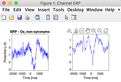
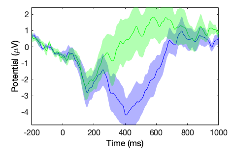
You may retrieve data by adding output variables as described in the help message of the std_erpplot.m function, and then replot it using the std_plotcurve function.
[STUDY erpdata erptimes] = std_erpplot(STUDY, ALLEEG, 'channels', {'Oz'}, 'timerange', [-200 1000]);
std_plotcurve(erptimes, erpdata, 'plotconditions', 'together', 'plotstderr', 'on', 'figure', 'on', 'filter', 30);
As shown above, the std_plotcurve.m function has additional parameters to plot the standard error which are not available from the EEGLAB graphic interface. The output of the function std_erpplot.m can also be controlled by the addition of parameters native to std_erpplot.m and pop_erpparams.m.
For example, notice the addition of the option timerange above to constrain the latency range to be between -200 to 1000ms.
Try some other commands from the channel plotting graphic interface and look at what is returned in the history (via the eegh.m function) to plot ERP in different formats.
Retrieving computed measures for subsequent processing
All STUDY plotting functions are able to return plotted results. After plotting STUDY results, look into the EEGLAB history (eegh from the MATLAB command line) to see which STUDY function was called, then look at the help of this function. It is usually possible to add additional parameters.
For example, if the following line appears in the EEGLAB history:
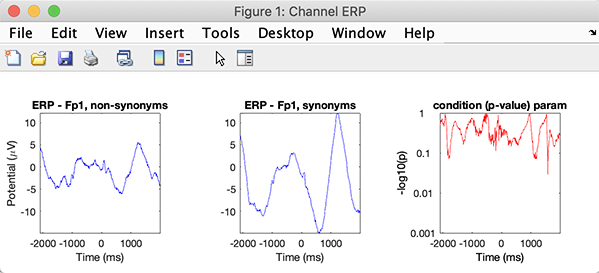
>> STUDY = std_erpplot(STUDY,ALLEEG,'channels',{ 'FP1'});
To retrieve results, add two outputs, one for the ERP data and one for the ERP time values, as follow:
>> [STUDY erpdata erptimes] = std_erpplot(STUDY,ALLEEG,'channels',{ 'FP1'}, 'noplot', 'on');
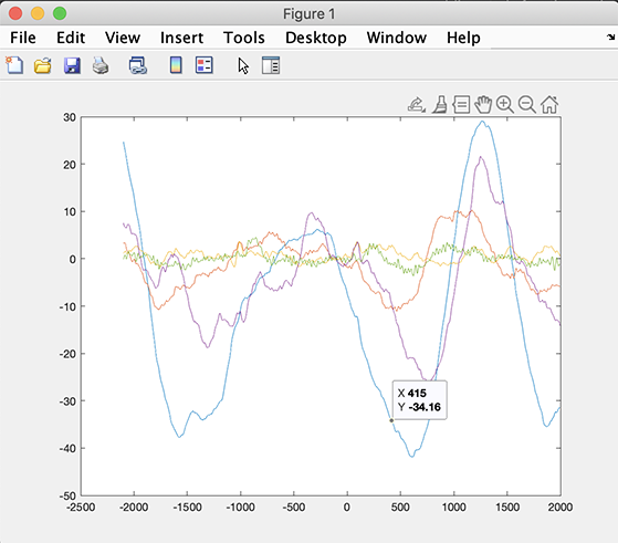
The erpdata array contains the ERP data for all subjects. Its size also depends on the STUDY design. The following command will plot the ERP for all subjects (included in the design) for the second cell in the STUDY design (the synonyms condition).
>> figure; plot(erptimes, erpdata{2});
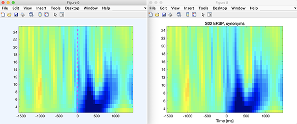
The small script below computes time-frequency decomposition on a small study. It also compares a time-frequency decomposition at the dataset level with a time-frequency decomposition at the STUDY level.
% Compute newtimef on first dataset for channel 1
options = {'freqscale', 'linear', 'freqs', [3 25], 'nfreqs', 20, 'ntimesout', 60, 'padratio', 1,'winsize',64,'baseline', 0};
TMPEEG = eeg_checkset(ALLEEG(1), 'loaddata');
figure; X = pop_newtimef( TMPEEG, 1, 1, [TMPEEG.xmin TMPEEG.xmax]*1000, [3 0.8] , 'topovec', 1, 'elocs', TMPEEG.chanlocs, 'chaninfo', TMPEEG.chaninfo, 'plotphase', 'off', options{:},'title',TMPEEG.setname, 'erspmax ',6.6);

% Compute newtimef for all datasets and plot first channel of first dataset
[STUDY, ALLEEG] = std_precomp(STUDY, ALLEEG, 'channels','recompute','on','ersp','on','erspparams',{'cycles' [3 0.8] 'parallel' 'on' options{:} },'itc','on');
STUDY = std_erspplot(STUDY,ALLEEG,'channels',{TMPEEG.chanlocs(1).labels}, 'subject', 'S02', 'design', 1 );
We should the result of the script below (after clicking on the plot to remove the side panels adjusting the color scale). It is not surprising that the result is the same since the same functions are being used in both cases.
Retrieving statistical results
All plotting functions able to compute statistics will return the statistical array in their output. You must first enable statistics either from the graphic interface or using a command-line call.
For instance to compute condition statistics, type:
>> STUDY = pop_statparams(STUDY, 'condstats', 'on');
Then, for a given channel, type:
>> [STUDY erpdata erptimes pgroup pcond pinter] = std_erpplot(STUDY,ALLEEG,'channels',{ 'FP1'});
Now, typing:
>> pcond

    pcond =
        [820x1]
The statistical array contains 820 p-values, one for each time point.
Note that the type of statistics returned depends on the parameter you selected in the ERP parameter graphic interface (for instance, if you selected permutation for statistics, the p-value based on surrogate data will be returned).
The pgroup and pinter arrays contain statistics across groups and the ANOVA interaction terms, respectively, if both groups and conditions are present.
Other functions such as std_specplot.m, std_erspplot.m, and std_itcplot.m behave in a similar manner (see the function help messages for more details). Note that for more control, you may also use directly call the statcond.m function, giving the erpdata cell array as input. See the help message of the statcond.m function for more help on this subject (see also example at the end of this page).
Saving results for processing in other software packages
Saving any STUDY result for subsequent processing in SPSS, Statistica, Stata, R, SAS, and Excel can easily be done from the command line. Saving a MATLAB array into a text file is simple in MATLAB. Below are five different options. All options are equivalent. Below we are saving the data for condition 1. Some save files with tab-separated values, while others save files with comma-separated values by default. Most functions below have many options.
array = erpdata{1}; % or array = rand(100,200);
dlmwrite('matlabarray1.txt',array,'delimiter', '\t', 'precision', 10); % tab separated values
xlswrite('matlabarray2.xls',array);
csvwrite('matlabarray3.csv',array); % comma separated values
writematrix(array, 'matlabarray4.csv');
writetable(table(array), 'matlabarray5.csv')
Imagine you have three conditions for ERP data of size 750 points x 13 subjects (erpdata obtained in the previous section). Imagine you have three conditions in the erpdata array. The short script below will save them in the file ‘erpfile.txt’ and append the condition in the last column. You may import this file into any statistical software and use the last column as the categorical predictor.
[STUDY erpdata erptimes] = std_erpplot(STUDY,ALLEEG,'channels',{ 'FP1'}, 'noplot', 'on');
dlmwrite('erpfile.txt',squeeze([ erptimes' erpdata{1} ones(size(erpdata{1},1),1)*1 ]),'delimiter', '\t', 'precision', 2);
dlmwrite('erpfile.txt',squeeze([ erptimes' erpdata{2} ones(size(erpdata{2},1),1)*2 ]),'-append', 'delimiter', '\t', 'precision', 2);
dlmwrite('erpfile.txt',squeeze([ erptimes' erpdata{3} ones(size(erpdata{3},1),1)*3 ]),'-append', 'delimiter', '\t', 'precision', 2);
The same goes if you have a set of n x m conditions. You can then add 2 columns representing 2 categorical variables.
dlmwrite('erpfile.txt',squeeze([ erpdata{1,1} ones(size(erpdata{1,1},1),1)*[1 1] ]),'delimiter', '\t', 'precision', 2);
dlmwrite('erpfile.txt',squeeze([ erpdata{1,2} ones(size(erpdata{1,2},1),1)*[1 2] ]),'-append', 'delimiter', '\t', 'precision', 2);
dlmwrite('erpfile.txt',squeeze([ erpdata{2,1} ones(size(erpdata{2,1},1),1)*[2 1] ]),'-append', 'delimiter', '\t', 'precision', 2);
dlmwrite('erpfile.txt',squeeze([ erpdata{2,2} ones(size(erpdata{2,2},1),1)*[2 2] ]),'-append', 'delimiter', '\t', 'precision', 2);
Imagine that you want to be able to use subjects as cases. in that case they cannot be defined as columns. Most statitical software will allow you convert between the two formats (they are usually called long and wide forms). In the case above, you would want to convert from wide to long form. Alternatlively, you may also use a MATLAB script. For example, for the erpdata condition 1 containing 750 points and 13 subjects, saving the data in long form would look like this. This file will only contain 2 columns, one for the data and one for the subject index.
dlmwrite('erpfile.txt',[ erpdata{1}(:,1) ones(size(erpdata{1},1),1)*1],'delimiter', '\t', 'precision', 2);
for iSubject = 2:size(erpdata{1},2)
    dlmwrite('erpfile.txt',squeeze([ erpdata{1}(:,iSubject) ones(size(erpdata{1},1),1)*iSubject]),'-append', 'delimiter', '\t', 'precision', 2);
end
Let’s look at a more general case of ERSP data. The script below can save ERSP data (ignore vs. memorize condition). The example below shows 12-time steps, 10 frequencies, 71 channels, and 13 subjects. More elegant and faster ways to do this exist.
chanlocs = eeg_mergelocs(ALLEEG.chanlocs);
[STUDY erspdata ersptimes erspfreqs] = std_erspplot(STUDY,ALLEEG,'channels',{chanlocs.labels}, 'noplot', 'on');
erspdata =

  2×1 cell array

    {10×12×71x13 single}
    {10×12×71x13 single}

if exist('erpfile.txt'), delete('erpfile.txt'); end
for iFreq = 1:10
  for iTime = 1:12
    for iChan = 1:71
      for iSubject = 1:13
          dlmwrite('erspfile.txt',squeeze([ erspdata{1}(iFreq,iTime,iSubject) iFreq iTime iChan iSubject 1]),'-append', 'delimiter', '\t', 'precision', 2);
          dlmwrite('erspfile.txt',squeeze([ erspdata{2}(iFreq,iTime,iSubject) iFreq iTime iChan iSubject 2]),'-append', 'delimiter', '\t', 'precision', 2);
      end
      end
  end
end
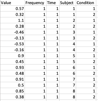
Below is the beginning of the saved file with the column names added. You may modify the script to add them as well automatically. This is just an example. Actual frequencies and time may be saved as well, replacing iFreq and iTime with erspfreqs(iFreq) and ersptimes(iTime) in the script above.
Computing and plotting component measures
Computing measures for components
The function pop_precomp.m can also be used to compute measures when working with components. As when working with channels, the function std_precomp.m can also precompute component measures. The syntax is very similar in both cases. For instance, the function pop_precomp.m called in the following way will launch the graphic user interface for computing measures on components:
[STUDY ALLEEG] = pop_precomp(STUDY, ALLEEG, 'components'); % pop up graphical interface
The same operation may be performed without the need to use the GUI when the function std_precomp.m is called with parameters defining the type of measure that wants to be computed. For example, in the following code snippet, ERP will be computed for all components:
[STUDY ALLEEG] = std_precomp(STUDY, ALLEEG, 'components', 'recompute', 'on', 'erp', 'on', 'filter', 30);
The type of measures computed are in close relationship with the hypothesis to be tested, and the selection of the measures technically constrains the type of analysis that can be performed. For instance, in the next section, the measures from each component will be aggregated to perform ICA component clustering. In the EEGLAB jargon, this is called pre-clustering. The measures used at the pre-clustering level have to be precomputed to be used for plotting. Then, ahead of pre-clustering, a careful assessment of the measures to be used and the parameters to use on its generation have to be carried.
Below is the code used for generating the measures:
[STUDY ALLEEG] = std_precomp(STUDY, ALLEEG, 'components',...
    'erp','on','erpparams',{'rmbase' [-200 0] },...
    'scalp','on',...
    'spec','on','specparams',{'freqrange' [3 50] 'specmode' 'fft' 'logtrials' 'off'},...
    'ersp','on','erspparams',{'cycles' [3 0.8] 'nfreqs' 100 'ntimesout' 200},...
    'itc','on');
Component pre-clustering and clustering
For clustering ICA components, we usually first compute all available activity measures. To specify clustering on power spectra in the [3 30]-Hz frequency range, ERPs in the [100 600]-ms time window, dipole location information (weighted by 10), and ERSP information with the above default values, type:
>> [STUDY ALLEEG] = std_preclust(STUDY, ALLEEG, 1,...
        {'spec' 'npca' 10 'weight' 1 'freqrange' [3 25] },...
        {'erp' 'npca' 10 'weight' 1 'timewindow' [100 600]  'erpfilter' '20'},...
        {'dipoles' 'weight' 10},...
        {'ersp' 'npca' 10 'freqrange' [3 25]  'timewindow' [-1600 1495]  'weight' 1 'norm' 1 'weight' 1});
Alternatively, to enter these values in the graphic interface, type:
>> [STUDY ALLEEG] = pop_preclust(STUDY, ALLEEG);
To cluster components from the command line, type:
>> [STUDY] = pop_clust(STUDY, ALLEEG, 'algorithm','kmeanscluster', 'clus_num', 10);
or to pop up the graphic interface:
>> [STUDY] = pop_clust(STUDY, ALLEEG);
Visualizing component clusters
The main function for visualizing component clusters is pop_clustedit.m. To pop up this interface, simply type:
>> [STUDY] = pop_clustedit(STUDY, ALLEEG);
This function calls a variety of plotting functions for plotting:
- scalp maps (std_topoplot.m),
- power spectra (std_specplot.m),
- equivalent dipoles (std_dipplot.m),
- ERPs (std_erpplot.m),
- ERSPs (std_erspplot.m),
- ITCs (std_itcplot.m).
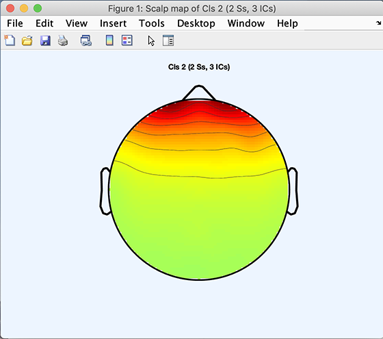
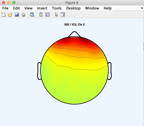
All of these functions follow the same calling format (though std_dipplot.m is slightly different; refer to its help message). Using function std_topoplot.m as an example, the following code will plot the average scalp map for cluster 2:
>> [STUDY] = std_topoplot(STUDY, ALLEEG, 'clusters', 2, 'mode', 'together');
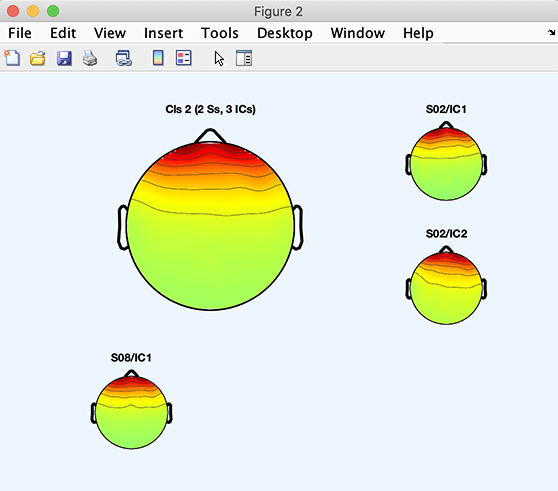
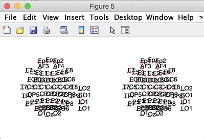
The code snippet below will plot the average scalp map for Cluster 3 plus the scalp maps of components belonging to Cluster 3:
>> [STUDY] = std_topoplot(STUDY, ALLEEG, 'clusters', 2, 'mode', 'apart');
The following code will plot component 3 of Cluster 2:
>> [STUDY] = std_topoplot(STUDY, ALLEEG, 'clusters', 2, 'comps', 3);
Computing and plotting custom measures
Computing custom measures
This section requires EEGLAB 2021.0 or later versions. It is possible to compute custom measures on STUDY using the std_precomp.m function. Before calling the custom function, the std_precomp.m function will conveniently apply dataset modifiers such as rmclust, rmicacomps or interp to remove components or interpolate channels. You may use the option customparam to pass additional parameters to your custom function.
First we call the function std_precomp.m to store the transformed single-trial data. For example, below, we remove the baseline (data samples from 1 to 410 out of 820). If you do not want to modify the single trials, then we can load them as explained later.
std_precomp(STUDY, ALLEEG, 'channels', 'customfunc', @(data)bsxfun(@minus, data, mean(data(:,1:410,:),2)), 'interp', 'on');
The code below low-pass filter the single-trial data below 10 Hz as another example of single trial processing.
std_precomp(STUDY, ALLEEG, 'channels', 'customfunc', @(data)reshape(eegfilt(data(:,:), EEG(1).srate, 0,10,EEG(1).pnts,60,0,'fir1'), size(data)), 'interp', 'on');
The we use the std_readata.m to import the processed data and organize it according to the selected STUDY design, in this case, two conditions synonyms versus non-synonyms. The data array for each condition is 820 time samples, 61 channels and 5 subjects.
[~, customdata] = std_readdata(STUDY, ALLEEG, 'channels', {ALLEEG(1).chanlocs.labels }, 'design', 1, 'datatype', 'custom');
customdata

  2×1 cell array
    {820×61×1×5 single}
    {820×61×1×5 single}
If you just want to read the unprocesed single-trial data organized according to the study design, read the ERP single-trial data as shown below. Note that the last dimension of the output arrays differs. This is because the custom function is for general purpose use and allows for 2-D array output for each channel (in which case the 3rd dimension will be larger than 1).
[~, erpdata] = std_readdata(STUDY, ALLEEG, 'channels', {ALLEEG(1).chanlocs.labels }, 'design', 1, 'datatype', 'erp');
erpdata

  2×1 cell array
    {820×61×5 single}
    {820×61×5 single}
Plotting custom measures
Then you can use the std_plotcurve.m to plot the data average. For example, the function below computes the ERP for each channel and plots it (either using the erpdata output array or using the customdata output array)
std_plotcurve(EEG(1).times, erpdata, 'chanlocs', ALLEEG(1).chanlocs);
customdata = cellfun(@squeeze, customdata, 'uniformoutput', false);
std_plotcurve(EEG(1).times, customdata, 'chanlocs', ALLEEG(1).chanlocs);
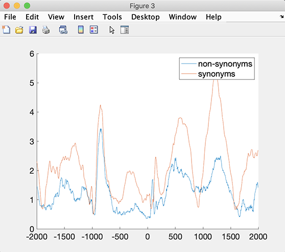
Or you can use your own function. For example, the code snippet below, computes the root mean square (RMS) across channels for each condition.
figure;
nCond = length(STUDY.design.variable(1).value);
for iCond = 1:nCond
  rms = sqrt(mean(mean(customdata{iCond},3).^2,2));
  hold on; plot(EEG(1).times, rms);
end
legend(STUDY.design.variable(1).value)
setfont(gcf, 'fontsize', 16); % change font size
Computing statistics on custom measures
Note that we can use the function std_stat.m to perform statistics on the customdata and customerp cell arrays obtained above. The code snippet below will use permutation statistics and false discovery correction for multiple comparisons. The output is an array of corrected p values of size 820 samples by 61 channels.
std_stat(erpdata, 'condstats', 'on', 'mcorrect', 'fdr', 'method', 'permutation')
ans =

  1×1 cell array
    {820×61 double}
The code snippet below performs correction for multiple comparisons using the cluster method available in FieldTrip.
std_stat(erpdata, 'condstats', 'on', 'fieldtripmcorrect', 'cluster', 'fieldtripmethod', 'montecarlo', 'mode', 'fieldtrip')
ans =

  1×1 cell array
    {820×61 double}
You may also call the low-level functions statcond.m and statcondfieldtrip.m directly (refer to the function help message for additional information). For example:
res = statcond(erpdata); size(res)
ans =
   820    61