The one sample t-test was computed on the contrasts faces vs scrambled faces, i.e. on differences. To fully appreciate the effect, we thus have to check differences on contrasts before looking at raw data.

Note that because we use a Bayesian confidence interval, we test directly H1 i.e. that the difference is not 0; which differs from the one-sample t-test that tests the null, if the difference is 0 (and the significant effect tells you the you should reject the hypothesis that this is 0 - still does not prove it is!).

Trimmed means of 1st level parameters

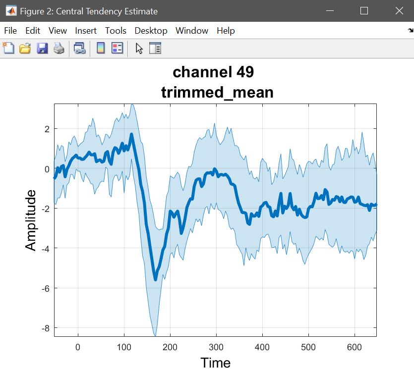
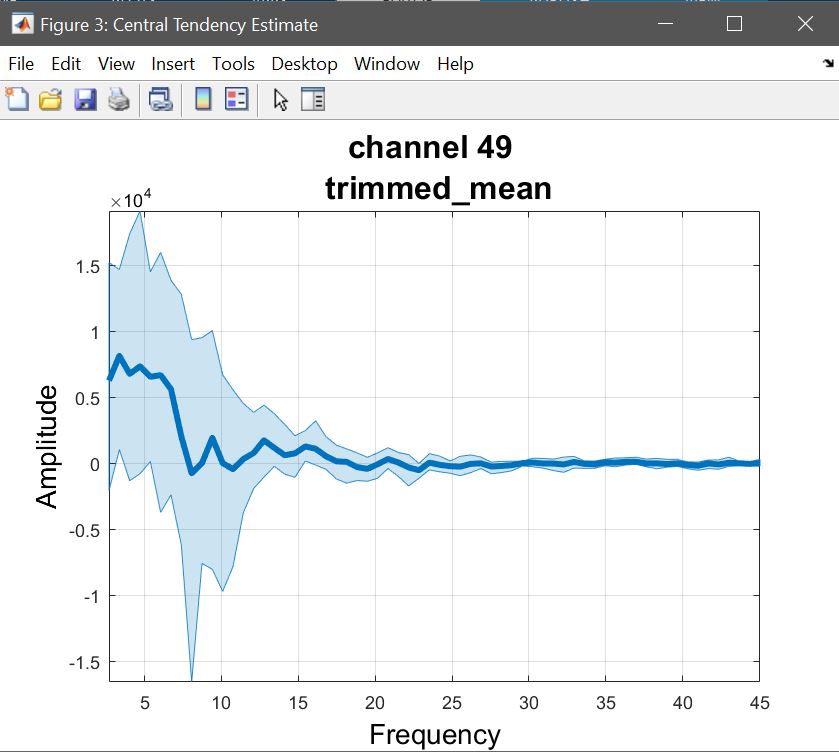
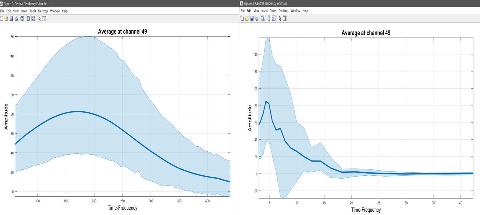
We start by computing the trimmed mean (because the t-test is on trimmed means) on the 1st level contrasts as we did before (figure 30 for ERP,Spectrum and ERSP), thus reflecting the t/p value maps.

Figure 30. TM ERP
Figure 30. TM Spectrum

Yr       = load('Yr.mat'); % this is the 1st level beta parameters 
chanlocs = [STUDY.filepath filesep 'limo_gp_level_chanlocs.mat'];
mkdir('average_betas'); cd('average_betas');
limo_central_tendency_and_ci(Yr.Yr, 'Trimmed mean',[],fullfile(pwd,'average.mat')); % could also use the text file as input
limo_add_plots('channel',49,fullfile(fileparts(pwd),'LIMO.mat'),...
    {fullfile(pwd,'average_Trimmed_mean.mat')}); title('Average at channel 49')
saveas(gcf, 'Average.fig'); close(gcf); cd ..

Figure 30. TM ERSP

Yr       = load('Yr.mat'); % this is the 1st level beta parameters 
chanlocs = [STUDY.filepath filesep 'limo_gp_level_chanlocs.mat'];
mkdir('average_betas'); cd('average_betas');
limo_central_tendency_and_ci(Yr.Yr, 'Trimmed mean',[],fullfile(pwd,'average.mat'))
limo_add_plots('channel',49,'restrict','time','dimvalue',5,fullfile(fileparts(pwd),'LIMO.mat'),...
    {fullfile(pwd,'average_Trimmed_mean.mat')}); title('Average at channel 49')
saveas(gcf, 'Average5Hz.fig'); close(gcf); 
limo_add_plots('channel',49,'restrict','frequency','dimvalue',180,fullfile(fileparts(pwd),'LIMO.mat'),...
    {fullfile(pwd,'average_Trimmed_mean.mat')}); title('Average at channel 49')
saveas(gcf, 'Average180ms.fig'); close(gcf);

Figure 30. Trimmed mean of contrasts faces>scrambled

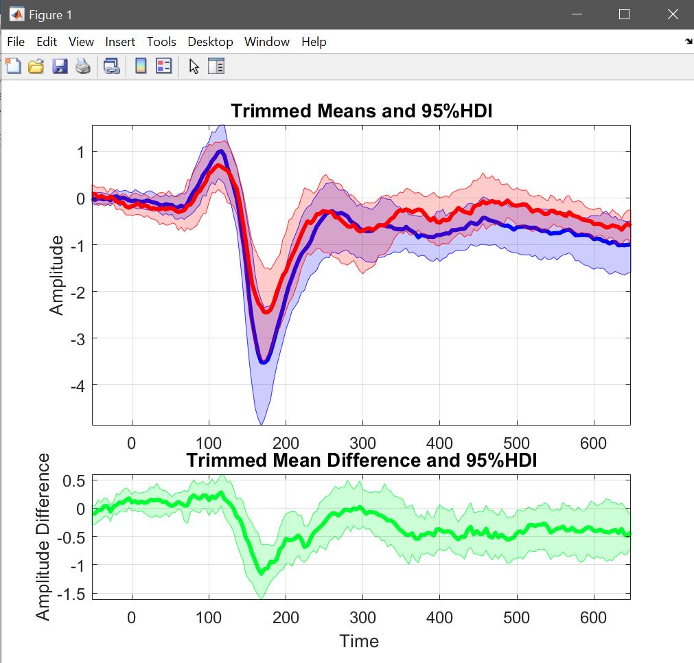
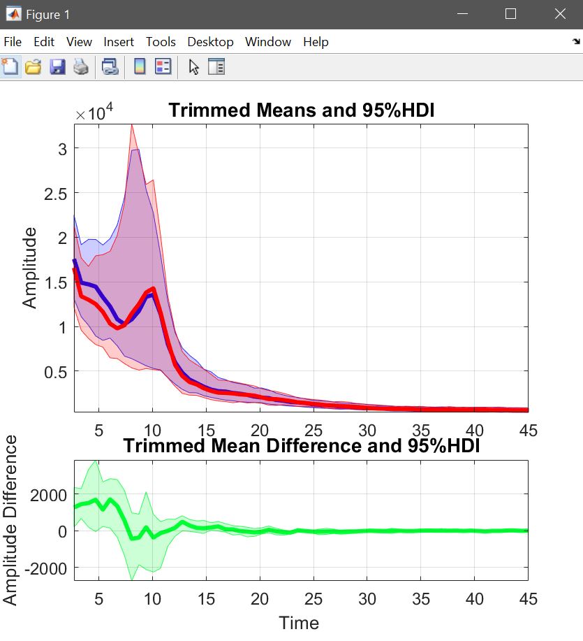
Trimmed mean differences of raw data

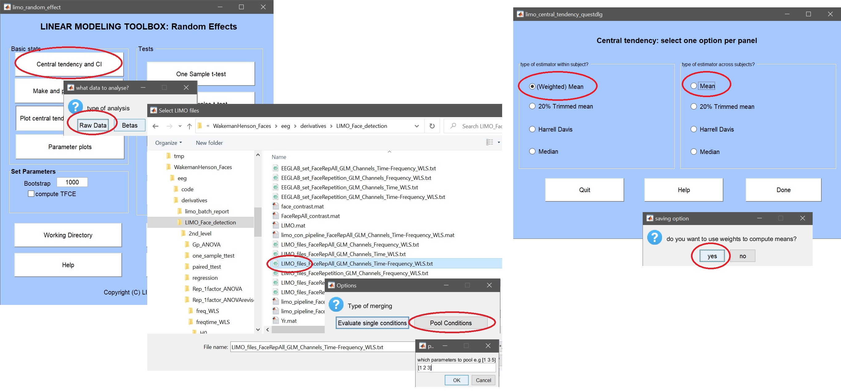
To look at the data, we compute the weighted mean for all famous and unfamiliar faces (pool conditions [1 2 3 7 8 9]) and for scrambled faces (pool conditions [4 5 6]) separately and use the trimmed mean across subjects (figure 26). Instead of visualizing each average, we can also Make and plot a difference, using the single subject’s data saved when computing averages (two files are saved the mean with CI and the single subjects, that’s what we use here). When plotting this, we can now see the difference directly with its confidence interval (figure 31 for ERP,Spectrum and ERSP). The saved file can of course seen again using plot central tendencies and differences.

Figure 31. TMD ERP
Figure 31. TMD Spectrum

% weighted mean for faces and scramble, followed by the difference
mkdir('Avg_data'); cd('Avg_data');
limo_central_tendency_and_ci(LIMOfiles, [1 2 3 7 8 9], chanlocs, 'Weighted mean', 'Mean', [],fullfile(pwd,'faces.mat'))  
limo_central_tendency_and_ci(LIMOfiles, [4 5 6], chanlocs, 'Weighted mean', 'Mean', [],fullfile(pwd,'scrambled.mat'))  
limo_plot_difference('faces_single_subjects_Weighted mean.mat','scrambled_single_subjects_Weighted mean',...
    'type','paired','name','faces_vs_scrambled','channel',49); % default 20% trimmed mean
saveas(gcf, 'Difference.fig'); close(gcf)

Figure 31. TMD ERSP

mkdir('ERSPs'); cd('ERSPs');
limo_central_tendency_and_ci(LIMOfiles, [1 2 3 7 8 9], chanlocs, 'Weighted mean', 'Mean', [],fullfile(pwd,'faces.mat'))  
limo_central_tendency_and_ci(LIMOfiles, [4 5 6], chanlocs, 'Weighted mean', 'Mean', [],fullfile(pwd,'scrambled.mat'))  
limo_plot_difference('faces_single_subjects_Weighted mean.mat','scrambled_single_subjects_Weighted mean',...
    'type','paired','name','faces_vs_scrambled','channel',49,'restrict','frequency'); % default 20% trimmed mean
saveas(gcf, 'DifferenceFreq.fig'); close(gcf)
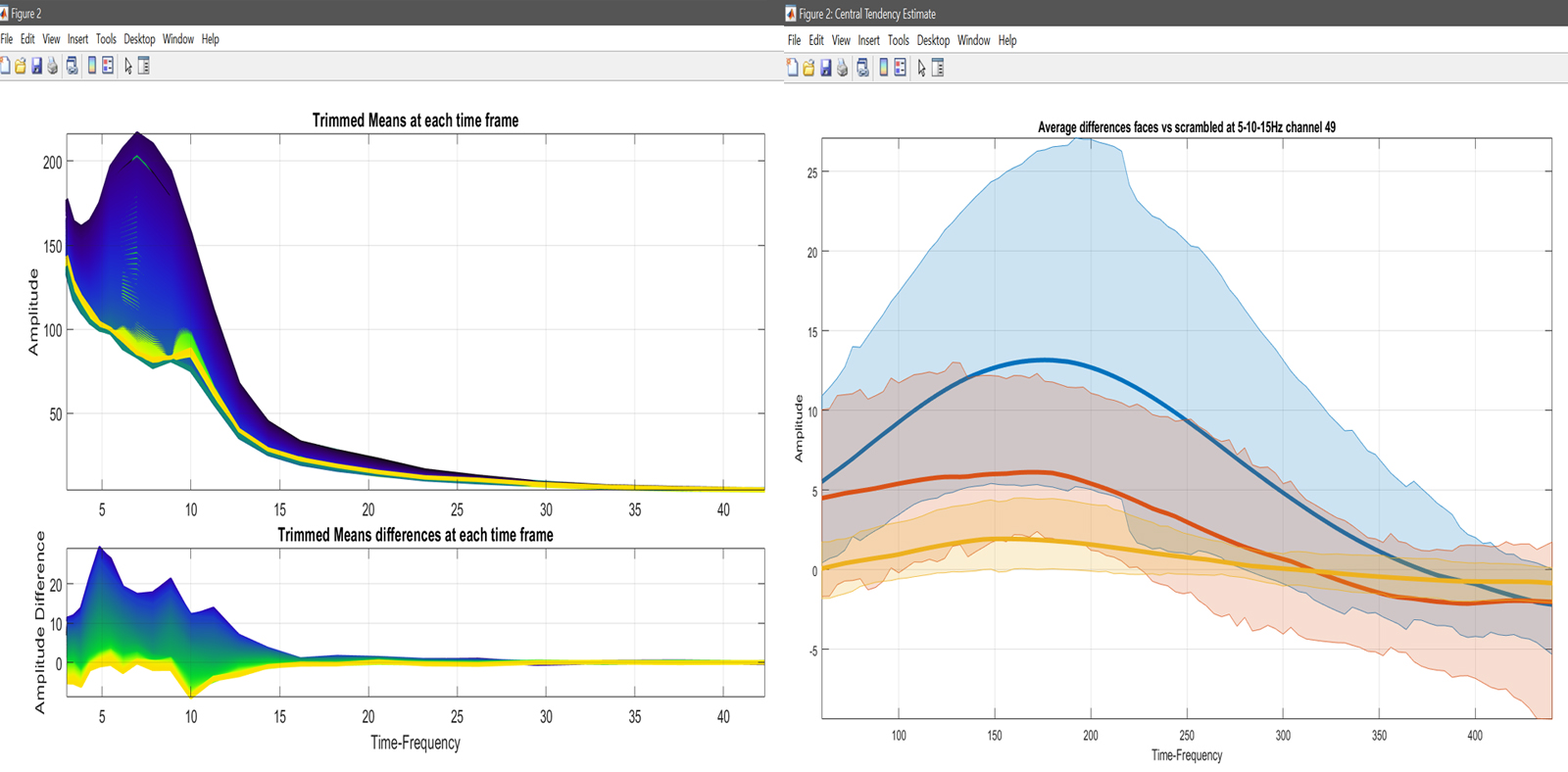
limo_add_plots('channel',49,'restrict','time','dimvalue',[5 10 15],fullfile(fileparts(pwd),'LIMO.mat'),...
    {fullfile(pwd,'faces_vs_scrambled.mat')}); % let's do channel 49 at 3 Frequencies
title('Average differences faces vs scrambled at 5-10-15Hz channel 49'); 
saveas(gcf, 'Difference5-10-15Hz.fig'); close(gcf)

Figure 31. Trimmed means of weighted means for faces and scrambled faces, and their trimmed mean difference.