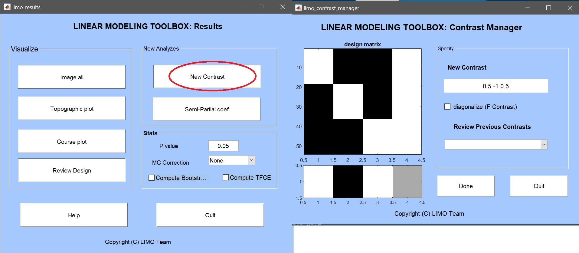
Let’s consider again the contrast of interest (Famous+Unfamiliar) Faces vs. Scrambled faces. This can be obtained from the 1-way ANOVA analysis, using a contrast [0.5 -1 0.5] (figures 16 - 17). This can also be obtained by computing this contrast per subject and performing a one sample t-test on this contrast. Since we have 9 conditions with the full design, the contrast is [0.5 0.5 0.5 -1 -1 -1 0.5 0.5 0.5]. To add one or many contrast, one must create a variable and save this as a file (while we could have a GUI, using a saved variable allows 1. to run many contrasts (each line is a new contrast to run) and 2. to be able to return and check this file a few weeks/months later after the analysis).

In the command window type:

C = [0.5 0.5 0.5 -1 -1 -1 0.5 0.5 0.5];
save('face_contrast','C')

In general, if the research question is a difference and/or interaction, there is no point doing a 2nd level ANOVA and it is recommended to pool conditions at the 1st level because there is less variance to account at the group level.

1st level contrast

From the LIMO main interface call the contrast manager and select to run the analysis on all subjects. Select the list of LIMO files to update and finally the contrast file (figure 28). LIMO will then compute the contrast for each subject, updating the LIMO.mat files and writing con files. A new list of con files is also created.

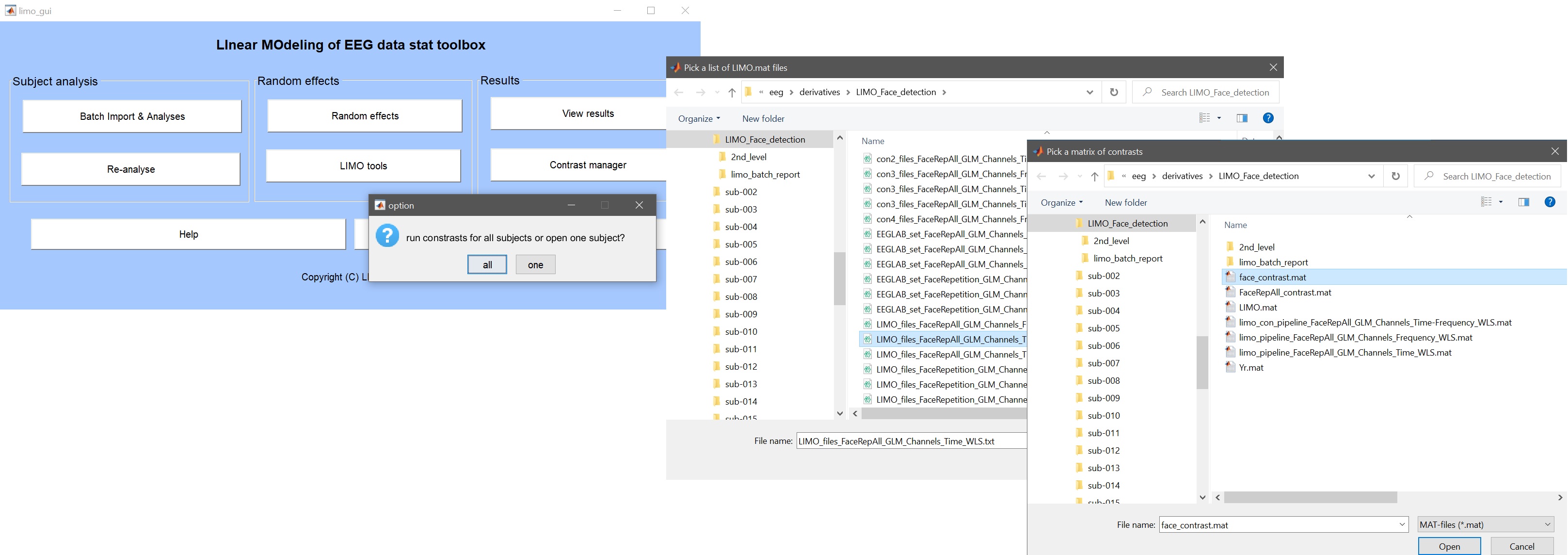Figure 28. GUI to create contrasts for all subjects from already computed models

Rather than loading a contrast into the GUI, we can pass all this info in command line (choosing your analysis ERP/Spectrum/ERSP):

cd(STUDY.filepath)
contrast.mat = [0.5 0.5 0.5 -1 -1 -1 0.5 0.5 0.5];
% ERP
[~,~,contrast.LIMO_files] = limo_get_files([],[],[],...
    fullfile(STUDY.filepath,['LIMO_' STUDY.filename(1:end-6)],'LIMO_files_FaceRepAll_GLM_Channels_Time_WLS.txt'));
% Spectrum
[~,~,contrast.LIMO_files] = limo_get_files([],[],[],...
    fullfile(STUDY.filepath,['LIMO_' STUDY.filename(1:end-6)],'LIMO_files_FaceRepAll_GLM_Channels_Frequency_WLS.txt'));
% ERSP
[~,~,contrast.LIMO_files] = limo_get_files([],[],[],...
    fullfile(STUDY.filepath,['LIMO_' STUDY.filename(1:end-6)],'LIMO_files_FaceRepAll_GLM_Channels_Time-Frequency_WLS.txt'));
limo_batch('contrast only',[],contrast)

2nd level

From the 2nd level GUI, select ‘one sample t-test’ and the new list of con files (should be con4 if you computed the revised ANOVA model). Once computations are done, using the result GUI and image all to see the results (figure 29 for ERP, Spectrum, and ERSP). Results are similar to the contrast in the one-way ANOVA but the number of clusters and/or significance differ.

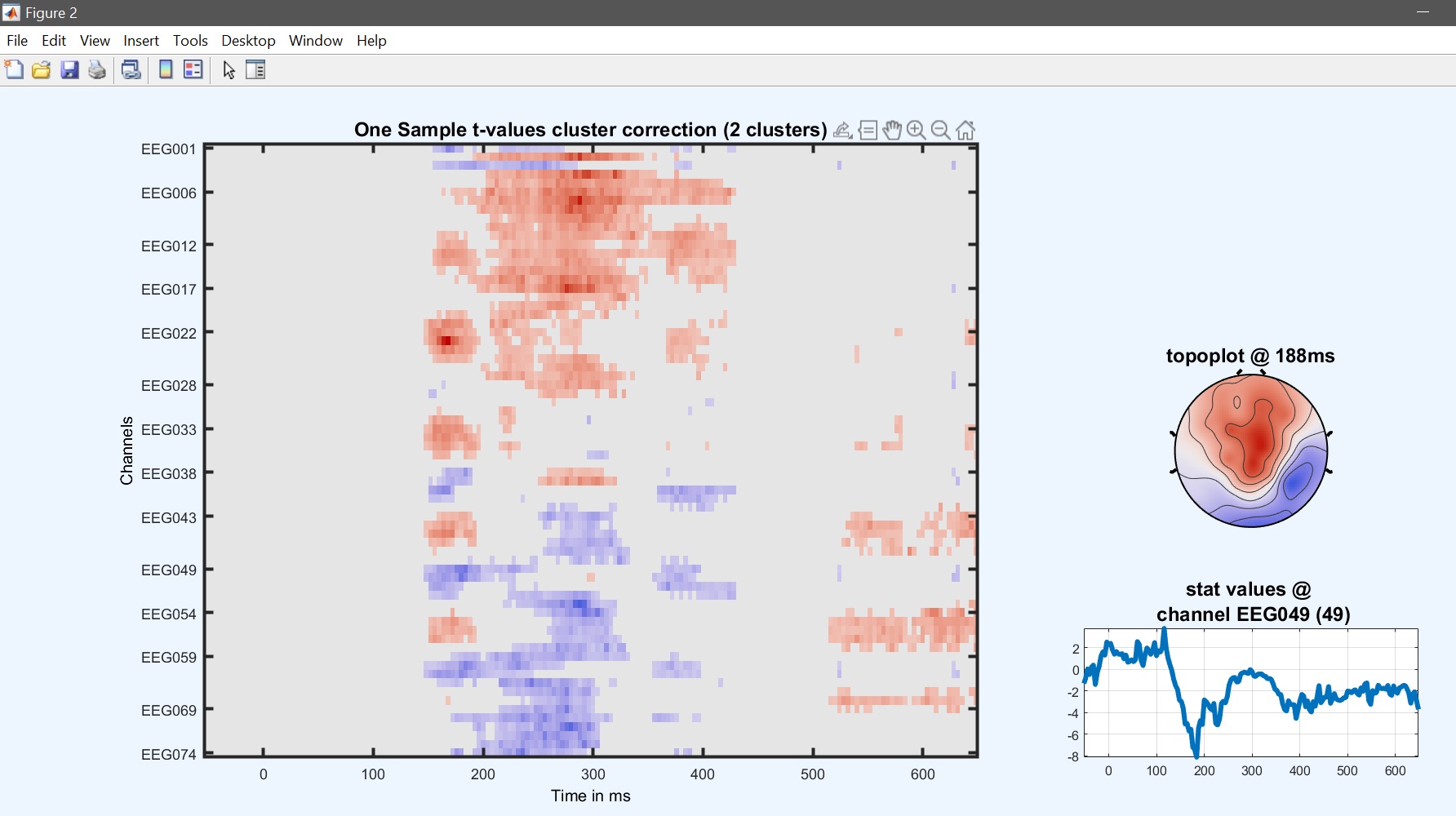
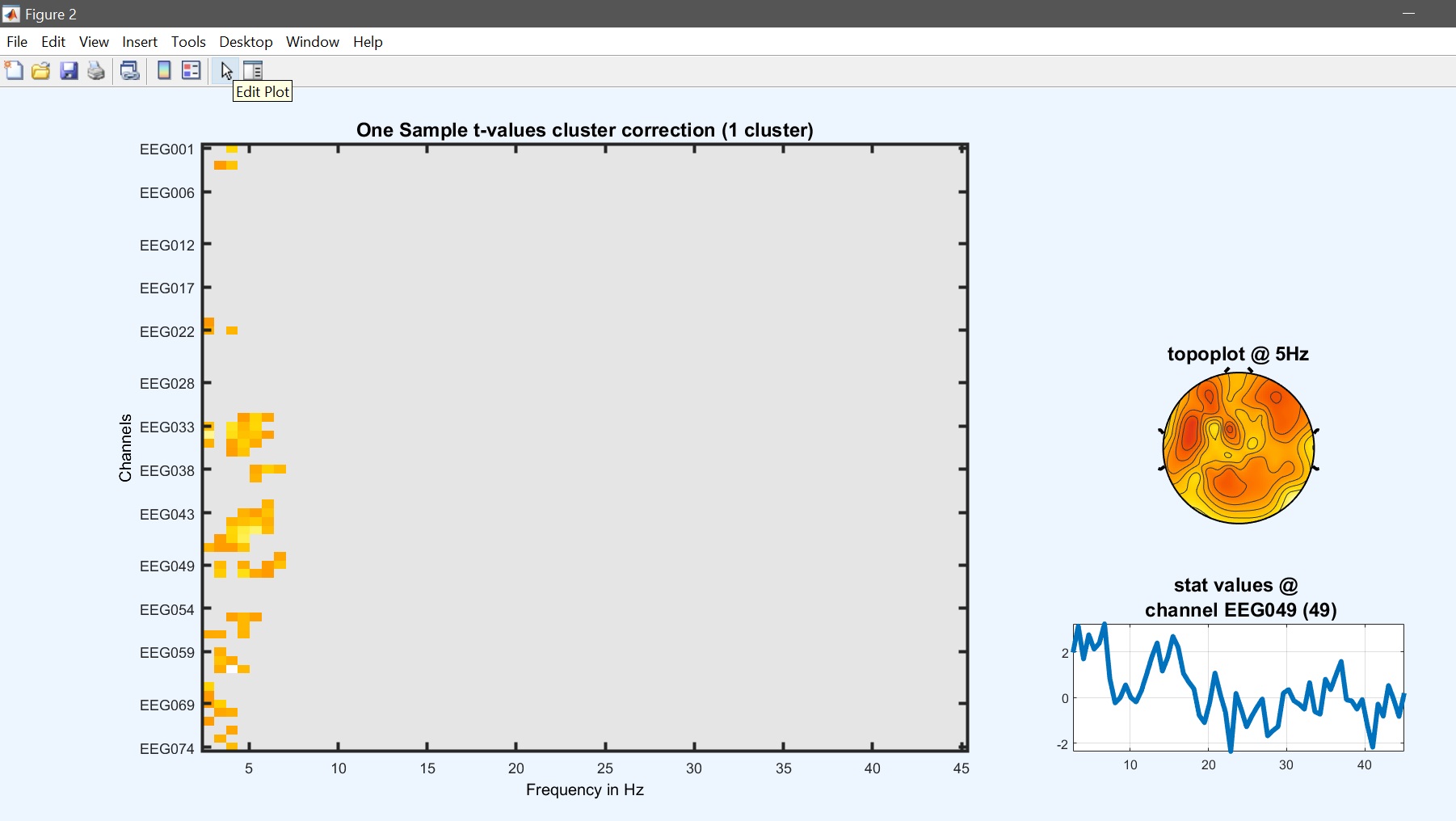
Figure 29. One-sample t-test on 1st level contrast

These steps can be executed in command line as:

chanlocs = [STUDY.filepath filesep 'limo_gp_level_chanlocs.mat'];
mkdir('one_sample'); cd('one_sample');
limo_random_select('one sample t-test',chanlocs,'LIMOfiles',...
    fullfile(STUDY.filepath,['LIMO_' STUDY.filename(1:end-6)],'con_4_files_FaceRepAll_GLM_Channels_Time_WLS.txt'),...
    'analysis_type','Full scalp analysis', 'type','Channels','nboot',101,'tfce',0);
limo_eeg(5,pwd)
limo_display_results(3,'one_sample_ttest_parameter_1.mat',pwd,0.05,2,...
    fullfile(pwd,'LIMO.mat'),0,'channels',49,'sumstats','mean'); % course plot
saveas(gcf, 'One_sample_timecourse.fig'); close(gcf)