Background on Independent Component Analysis applied to EEG
This appendix gives background information and more details on ICA in general as well as on ICA algorithms available using EEGLAB. For practical information on how to run ICA using EEGLAB please refer to the tutorial sections dealing with running ICA decompositions and plotting ICA decompositions.
Independent Component Analysis of EEG data
Decomposing data by ICA (or any linear decomposition method, including PCA and its derivatives) involves a linear change of basis from data collected at single scalp channels into a spatially transformed “virtual channel” basis.
That is, instead of a collection of simultaneously recorded single-channel data records, the data are transformed to a collection of simultaneously recorded outputs of spatial filters applied to the whole multi-channel data. These spatial filters may be designed in many ways for many purposes.
In the original scalp channel data, each row of the data recording matrix represents the time course of summed in voltage differences between source projections to one data channel and one or more reference channels (thus itself constituting a linear spatial filter). After ICA decomposition, each row of the data activation matrix gives the time course of the activity of one component process spatially filtered from the channel data.
In the case of ICA decomposition, the independent component filters are chosen to produce the maximally temporally independent signals available in the channel data. These are, in effect, information sources in the data whose mixtures, via volume conduction, have been recorded at the scalp channels. The mixing process (for EEG, by volume conduction) is passive, linear, and adds no information to the data. On the contrary, it mixes and obscures the functionally distinct and independent source contributions.
These information sources may represent synchronous or partially synchronous activity within one (or possibly more) cortical patch(es), else activity from non-cortical sources (e.g., potentials induced by eyeball movements or produced by single muscle activity, line noise, etc.). The following example shows the diversity of source information typically contained in EEG data and the striking ability of ICA to separate out these activities from the recorded channel mixtures.
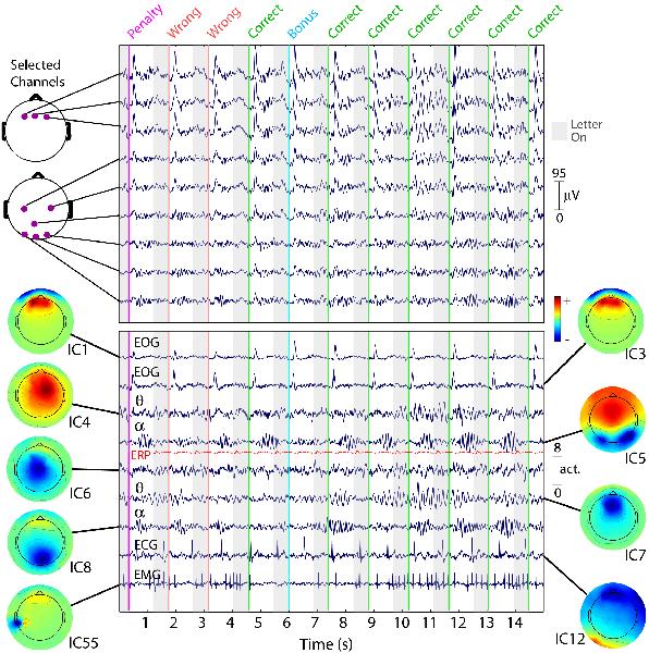
Fifteen seconds of EEG data at 9 (of 100) scalp channels (top panel) with activities of 9 (of 100) independent components (ICs, bottom panel). While nearby electrodes (upper panel) record highly similar mixtures of brain and non-brain activities, ICA component activities (lower panel) are temporally distinct (i.e., maximally independent over time), even when their scalp maps are overlapping. Compare, for example, IC1 and IC3, accounting for different phases of eye blink artifacts produced by this subject after each visual letter presentation (grey background) and ensuing auditory performance feedback signal (colored lines). Compare, also, IC4 and IC7, which account for overlapping frontal (4-8 Hz) theta band activities appearing during a stretch of correct performance (seconds 7 through 15). Typical ECG and EMG artifact ICs are also shown, as well as overlapping posterior (8-12 Hz) alpha band bursts that appear when the subject waits for the next letter presentation (white background). For comparison, the repeated average visual evoked response of a bilateral occipital IC process (IC5) is shown (in red) on the same (relative) scale. Clearly, the unaveraged activity dynamics of this IC process are not well summarized by its averaged response, a dramatic illustration of the independence of phase-locked and phase-incoherent activity. From Onton and Makeig, 2006.
Note on ICA algorithms
Applied to simulated, relatively low dimensional data sets for which all the assumptions of ICA are exactly fulfilled, all three algorithms return near-equivalent components. We are satisfied that Infomax ICA (runica) gives stable decompositions with up to hundreds of channels (assuming enough training data are given, see below), and therefore we can recommend its use. We have also tested the physiological significance of any differences in the results or different algorithms in Delorme et al., 2012. We have shown that all tested ICA algorithms return similar decompositions.
Note about jader: This algorithm uses 4th-order moments (whereas Infomax uses (implicitly) a combination of higher-order moments), but the storage required for all the 4th-order moments becomes impractical for datasets with more than ~50 channels.
Note about fastica: This algorithm quickly computes individual components (one by one) when used with its default parameters. However, the order of the components it finds cannot be known in advance, and performing a complete decomposition is not necessarily faster than Infomax. Thus for practical purposes its name for it should not be taken literally. Also, in our experience it may be less stable than Infomax for high-dimensional data sets.
How many data points do I need to run an ICA?
As a general rule, finding N stable components (from N-channel data) typically requires more than kN^2 data sample points (at each channel), where N^2 is the number of weights in the unmixing matrix that ICA is trying to learn and k is a multiplier. In our experience, the value of k increases as the number of channels increases. In our example using 32 channels, we have 30800 data points, giving 30800/32^2 = 30 pts/weight points. However, to find 256 components, it appears that even 30 points per weight is not enough data.
Can you use too much data? The short answer is no. However, suppose you have two tasks in your experiment and are planning to process them separately (for two papers, for example). In that case, it is probably better to run ICA on them separately because they may contain different ICA brain components. Because the number of components is limited to the number of channels, processing the two tasks together might mean that you might have fewer components specific to each task. Also, if you have different sessions for the same subject (data collected on different days), these should be processed separately because of the slightly different electrode placements.
ICA weights
In the command line printout here, the angledelta is the angle between the direction of the vector in weight space describing the current learning step and the direction describing the previous step. An intuitive view of the annealing angle (angledelta) threshold (see above) is as follows: If the learning step takes the weight vector (in global weight vector space) ‘past’ the true or best solution point, the following step will have to ‘back-track.’ Therefore, the learning rate is too high (the learning steps are too big) and should be reduced. If, on the other hand, the learning rate were too low, the angle would be near 0 degrees, learning would proceed in (small) steps in the same direction, and learning would be slow. The default annealing threshold of 60 degrees was arrived at heuristically and might not be optimum.
The runica Infomax function returns two matrices, a data sphering matrix (which is used as a linear preprocessing to ICA) and the ICA weight matrix. For more information, refer to ICA help pages (i.e., ICA basic theory). If you wish, the resulting decomposition (i.e., ICA weights and sphere matrices) can then be applied to longer epochs drawn from the same data, e.g., for time-frequency decompositions for which epochs of 3-sec or more may be desirable.
Differences between ICA and PCA
The component order returned by runica is in decreasing order of the EEG variance accounted for by each component. In other words, the lower the order of a component, the more data (neural and/or artifactual) it accounts for. In contrast to PCA, for which the first component may account for 50% of the data, the second 25%, etc., ICA component contributions are much more homogeneous, ranging from roughly 5% down to ~0%. This is because PCA specifically makes each successive component account for as much as possible of the remaining activity not accounted for by previously determined components – while ICA seeks maximally independent sources of activity.
PCA components are temporally or spatially orthogonal - smaller component projections to scalp EEG data typically looking like checkerboards - while ICA components of EEG data are maximally temporally independent but spatially unconstrained – and therefore able to find maps representing the projection of a partially synchronized domain / island / patch / region of cortex, no matter how much it may overlap the projections of other (relatively independent) EEG sources. This is useful since, apart from ideally (radially) oriented dipoles on the cortical surface (i.e., on cortical gyri, not in sulci), simple biophysics shows that the volume projection of each cortical domain must project appreciably to much of the scalp.