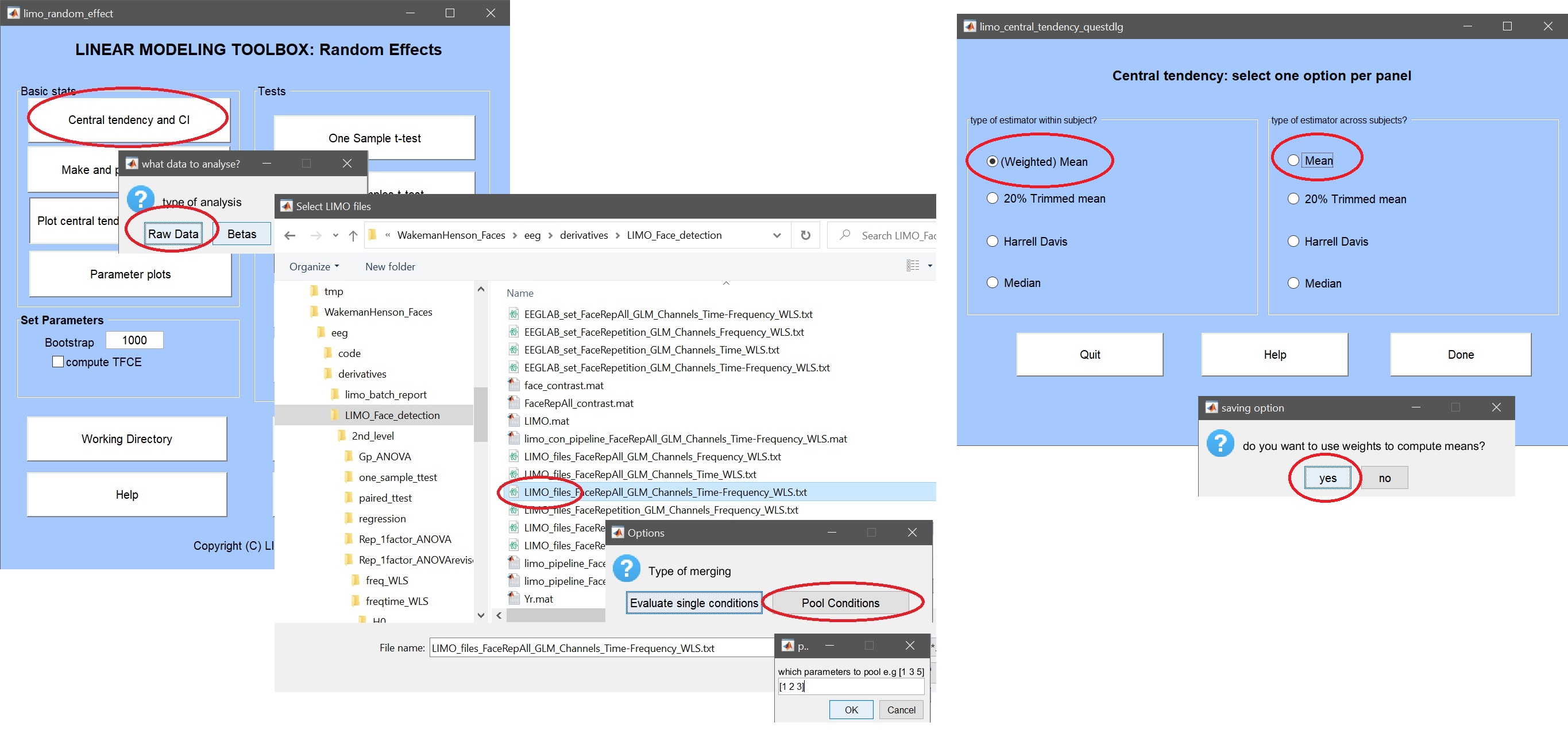
Statistics course plot
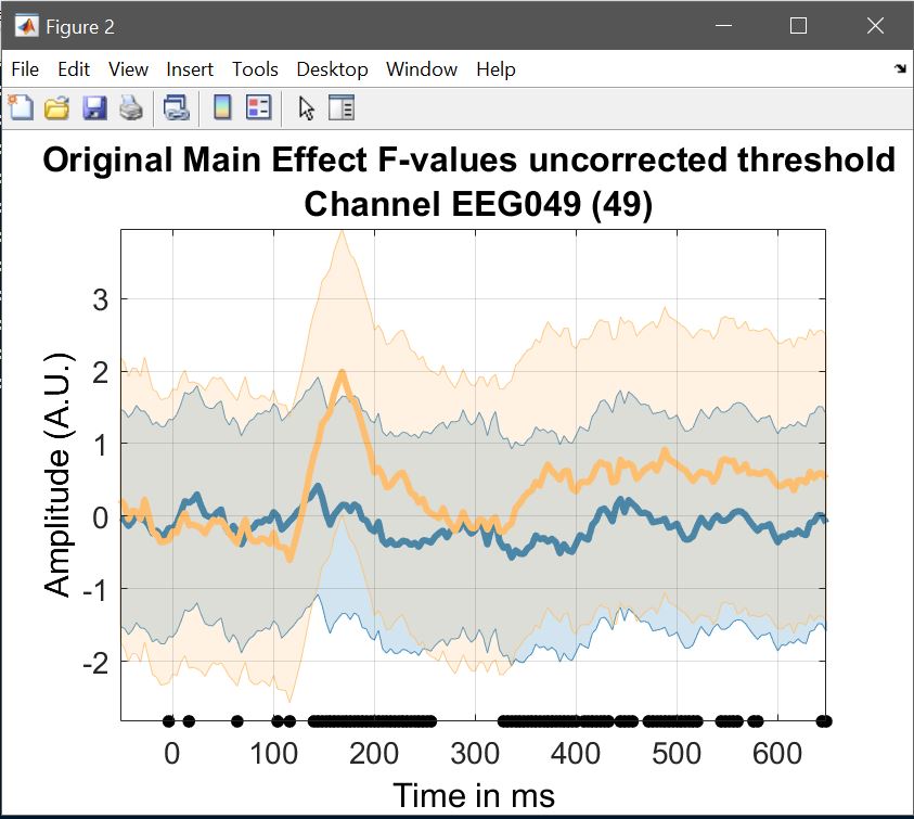
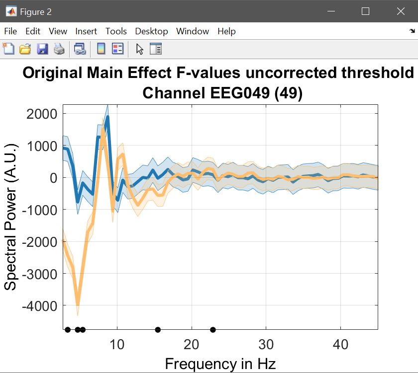
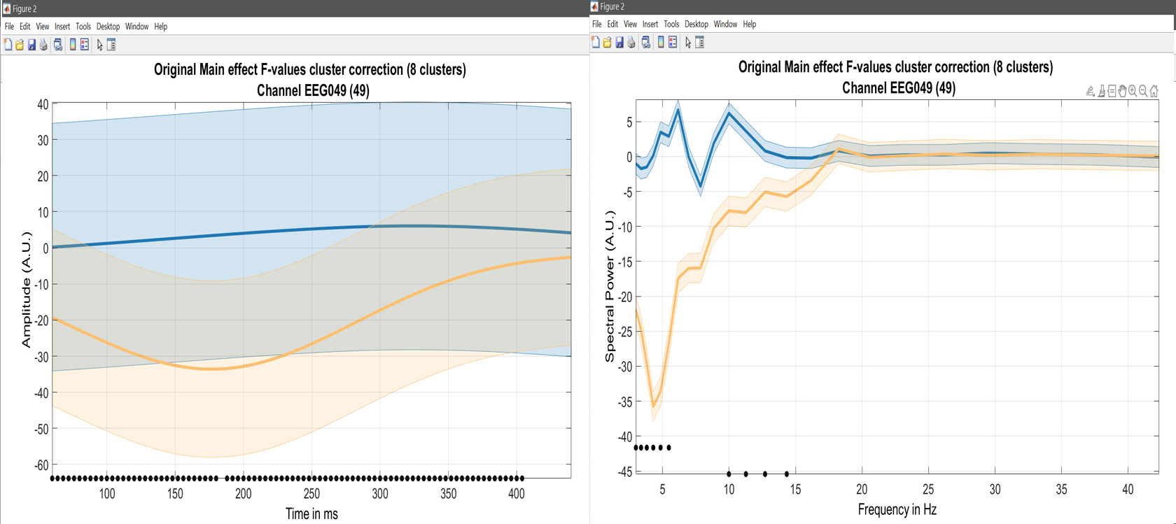
When it comes to statistical results, ‘image all’ gives you all F and p-values, and clusters (if computed), ‘course plot’ also shows the time course of the effects for a specified channel. In a 1-way ANOVA, this would typically be only 2 curves for 3 conditions, because the F test involves only two simultaneous contrasts (if we know A>B and B>C then we know A>C and the actual statistical test doesn’t need to compute all differences). For a contrast, this is only 1 curve, testing if the (trimmed) mean difference equal to 0 (e.g. figure 17).
Here, after computing a one-way ANOVA, we can check this is the case, type: load('LIMO.mat'); LIMO.design.C{1} and the result is a matrix which tested for mean differences between familiar and unfamiliar faces and between scrambled and unfamiliar faces ([1 0 -1; 0 1 -1]), giving in the course plot 2 curves – (figure 23 for ERP, spectrum and ERSP).
limo_display_results(3,'Rep_ANOVA_Main_effect_1_face.mat',pwd,0.05,2,...
    fullfile(pwd,'LIMO.mat'),0,'channels',49,'sumstats','mean'); % course plot
saveas(gcf, 'Rep_ANOVA_Main_effect_timecourse.fig'); close(gcf)
limo_display_results(3,'Rep_ANOVA_Main_effect_1_face.mat',pwd,0.05,2,...
    fullfile(pwd,'LIMO.mat'),0,'channels',49,'sumstats','mean'); % spectrum plot
saveas(gcf, 'Rep_ANOVA_Main_effect_spectrum.fig'); close(gcf)
limo_display_results(3,'Rep_ANOVA_Main_effect_1_face.mat',pwd,0.05,2,...
    fullfile(pwd,'LIMO.mat'),0,'channels',49,'restrict','time','dimvalue',5,'sumstats','mean'); % course plot
saveas(gcf, 'Rep_ANOVA_Main_effect_5Hztimecourse.fig'); close(gcf)
limo_display_results(3,'Rep_ANOVA_Main_effect_1_face.mat',pwd,0.05,2,...
    fullfile(pwd,'LIMO.mat'),0,'channels',49,'restrict','frequency','dimvalue',180,'sumstats','mean'); % course plot
saveas(gcf, 'Rep_ANOVA_Main_effect_180msSpectrum.fig'); close(gcf)
Figure 23. Course plot of the ANOVA
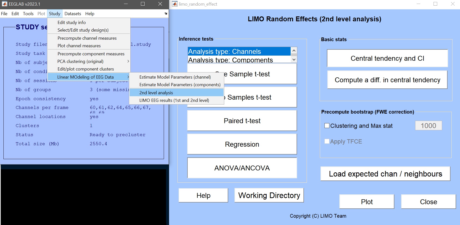
It is however also important to relate results to the data. For that, we can compute averages and check on effect sizes. This can be achieved from the 2nd level menu (figure 9) through the ‘basic stats’ submenu.
Statistics effect sizes
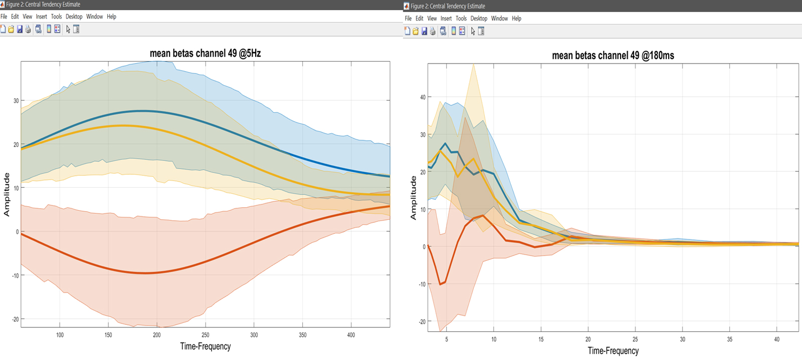
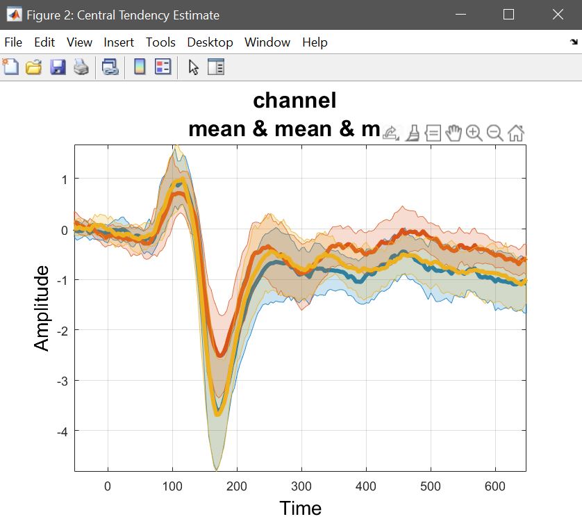
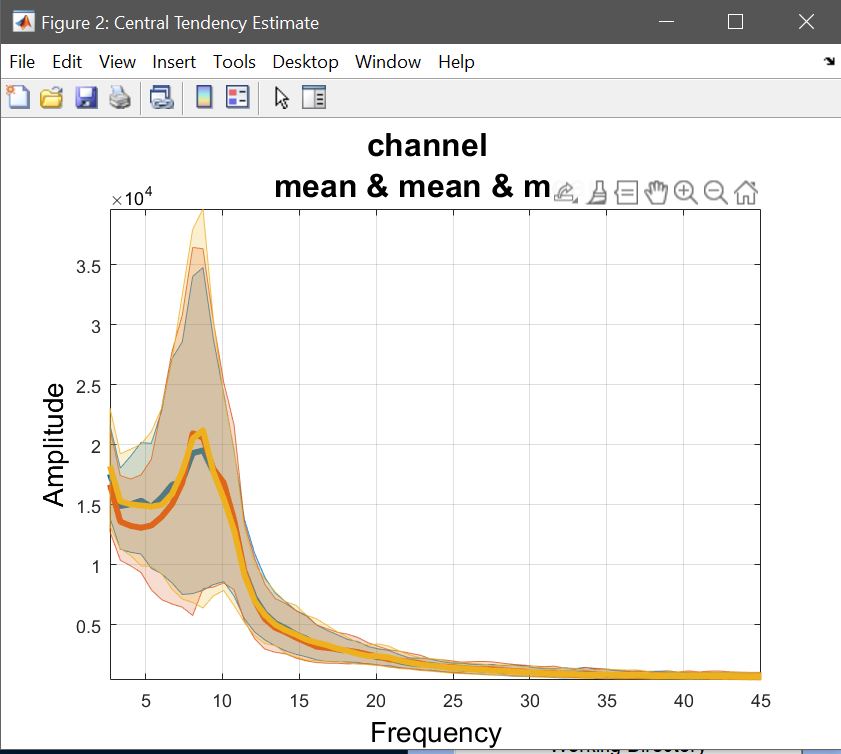
The 2nd level ANOVA is computed on beta parameters, or a linear combination, i.e. contrasts. The means with confidence intervals can be computed using LIMO, chosing Central tendency and CI. Repeated measures ANOVA being computed on means, here we compute the mean of each contrasts (i.e. selecting the list for con1, and repeating for con2 and con3) – you can choose do compute for all channels or just one (figure 24). Use plot central tendency and differences to visualize the results – figure 25 for ERP, spectrum and ERSP.
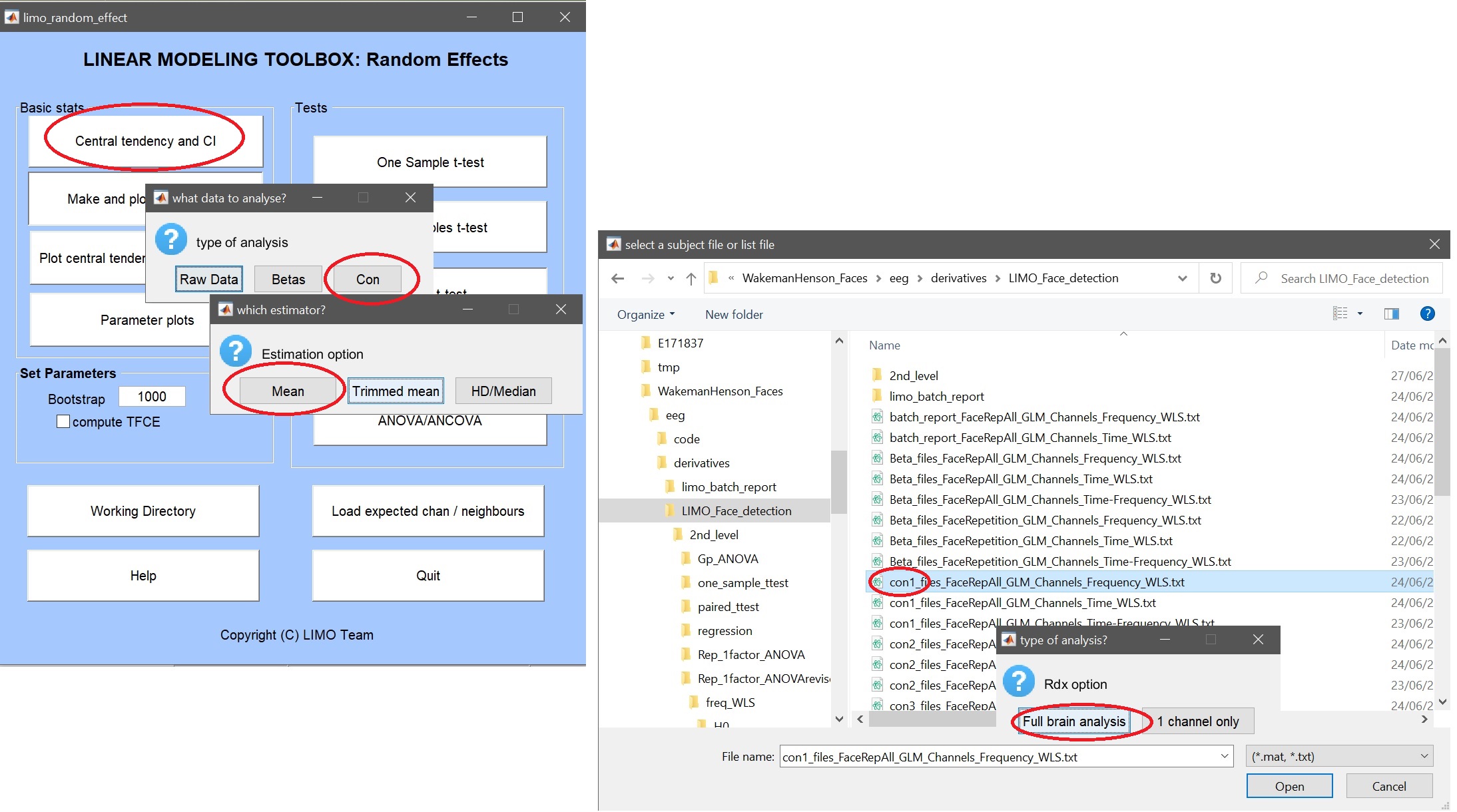
Figure 24. GUI for Central tendency and CI, selecting data type (e.g. con), summary statistics (e.g. mean), files or list (.txt) of files and the channels (e.g. full brain).
Yr       = load('Yr.mat'); % ANOVA data are channel*[freq/time]frames*subjects*conditions
chanlocs = [STUDY.filepath filesep 'limo_gp_level_chanlocs.mat'];
mkdir('average_betas'); cd('average_betas');
limo_central_tendency_and_ci(squeeze(Yr.Yr(:,:,:,1)), 'Mean',[],fullfile(pwd,'famous.mat'))
limo_central_tendency_and_ci(squeeze(Yr.Yr(:,:,:,2)), 'Mean',[],fullfile(pwd,'scrambled.mat'))
limo_central_tendency_and_ci(squeeze(Yr.Yr(:,:,:,3)), 'Mean',[],fullfile(pwd,'unfamiliar.mat'))
limo_add_plots('channel',49,fullfile(fileparts(pwd),'LIMO.mat'),...
    {fullfile(pwd,'famous_Mean.mat'), fullfile(pwd,'scrambled_Mean.mat'), fullfile(pwd,'unfamiliar_Mean.mat')})
title('mean betas channel 49'); saveas(gcf, 'Rep_ANOVA_Main_effect_Betas.fig'); close(gcf)
Yr       = load('Yr.mat'); % ANOVA data are channel*[freq/time]frames*subjects*conditions
chanlocs = [STUDY.filepath filesep 'limo_gp_level_chanlocs.mat'];
mkdir('average_betas'); cd('average_betas');
limo_central_tendency_and_ci(squeeze(Yr.Yr(:,:,:,:,1)), 'Mean',[],fullfile(pwd,'famous.mat'))
limo_central_tendency_and_ci(squeeze(Yr.Yr(:,:,:,:,2)), 'Mean',[],fullfile(pwd,'scrambled.mat'))
limo_central_tendency_and_ci(squeeze(Yr.Yr(:,:,:,:,3)), 'Mean',[],fullfile(pwd,'unfamiliar.mat'))
limo_add_plots('channel',49,'restrict','time','dimvalue',5,fullfile(fileparts(pwd),'LIMO.mat'),...
    {fullfile(pwd,'famous_Mean.mat'), fullfile(pwd,'scrambled_Mean.mat'), fullfile(pwd,'unfamiliar_Mean.mat')})
title('mean betas channel 49 @5Hz'); saveas(gcf, 'Rep_ANOVA_Main_effect_Betas5Hz.fig'); close(gcf)
limo_add_plots('channel',49,'restrict','frequency','dimvalue',180,fullfile(fileparts(pwd),'LIMO.mat'),...
    {fullfile(pwd,'famous_Mean.mat'), fullfile(pwd,'scrambled_Mean.mat'), fullfile(pwd,'unfamiliar_Mean.mat')})
title('mean betas channel 49 @180ms'); saveas(gcf, 'Rep_ANOVA_Main_effect_Betas180ms.fig'); close(gcf)
Figure 25. Mean con values.
Raw data effect sizes
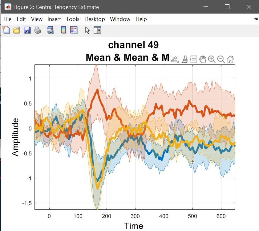
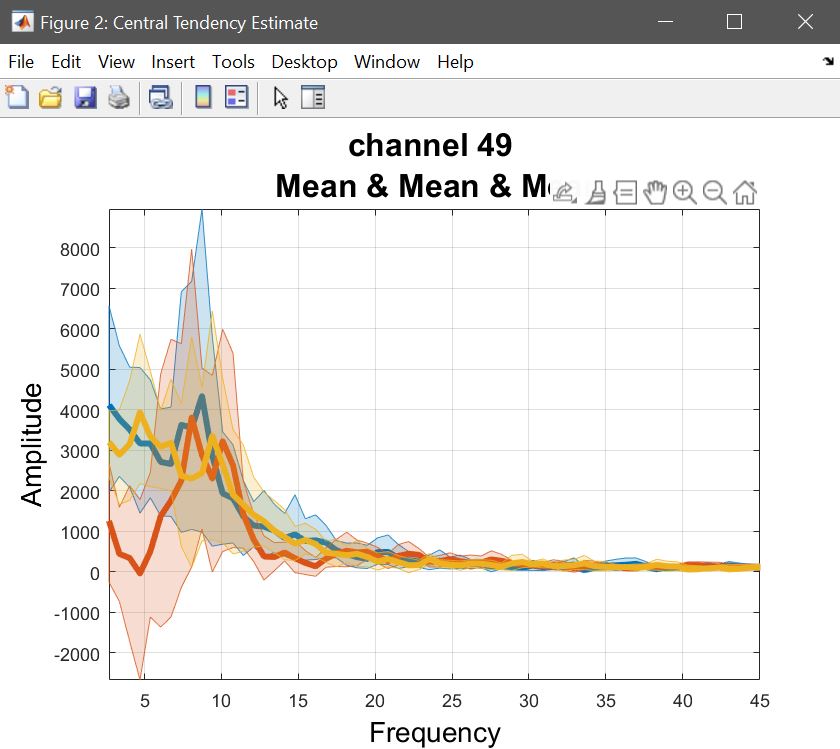
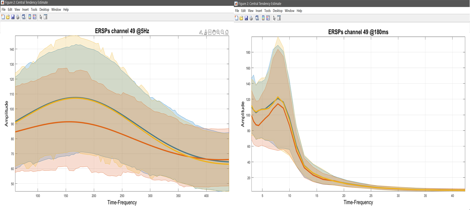
While computing the means or trimmed means of betas/cons (1) reflects the computations done at the 2nd level, and (2) allows to understand results, it doesn’t show the underlying data and raw effect sizes, needed to interpret results. This means we want to compute Central tendency and CI on ‘Raw Data’ (understand pre-processed – figure 26). Select a list of LIMO files, and select to pool conditions – [1 2 3] for famous faces, [4 5 6] for scrambled faces, and [7 8 9] for unfamiliar faces. You have the option to just do it for a channel of interest or the full brain analysis, and then use your estimators. Here, we want to see the means of each condition, using the weights from each trials (since at the 1st level we used WLS). This needs to be repeated for every condition. Using ‘plot central tendencies and differences’ of the 2nd level menu or the ‘course plot’ of the result menu, you can plot those averages. Results are shown figure 27 for ERP, Spectrum and ERSP.
LIMOfiles = fullfile(STUDY.filepath,['LIMO_' STUDY.filename(1:end-6)],'LIMO_files_FaceRepAll_GLM_Channels_Time_WLS.txt');
mkdir('ERPs'); cd('ERPs');
limo_central_tendency_and_ci(LIMOfiles, [1 2 3], chanlocs, 'Weighted mean', 'Mean', [],fullfile(pwd,'famous.mat'))
limo_central_tendency_and_ci(LIMOfiles, [4 5 6], chanlocs, 'Weighted mean', 'Mean', [],fullfile(pwd,'scrambled.mat'))
limo_central_tendency_and_ci(LIMOfiles, [7 8 9], chanlocs, 'Weighted mean', 'Mean', [],fullfile(pwd,'unfamiliar.mat'))
limo_add_plots('channel',49,fullfile(fileparts(pwd),'LIMO.mat'),...
    {fullfile(pwd,'famous_Mean_of_Weighted mean.mat'),fullfile(pwd,'scrambled_Mean_of_Weighted mean.mat'),...
    fullfile(pwd,'unfamiliar_Mean_of_Weighted mean.mat')}); title('ERPs channel 49')
saveas(gcf, 'Rep_ANOVA_Main_effectERP.fig'); close(gcf)
LIMOfiles = fullfile(STUDY.filepath,['LIMO_' STUDY.filename(1:end-6)],'LIMO_files_FaceRepAll_GLM_Channels_Frequency_WLS.txt');
mkdir('ERPs'); cd('ERPs');
limo_central_tendency_and_ci(LIMOfiles, [1 2 3], chanlocs, 'Weighted mean', 'Mean', [],fullfile(pwd,'famous.mat'))
limo_central_tendency_and_ci(LIMOfiles, [4 5 6], chanlocs, 'Weighted mean', 'Mean', [],fullfile(pwd,'scrambled.mat'))
limo_central_tendency_and_ci(LIMOfiles, [7 8 9], chanlocs, 'Weighted mean', 'Mean', [],fullfile(pwd,'unfamiliar.mat'))
limo_add_plots('channel',49,fullfile(fileparts(pwd),'LIMO.mat'),...
    {fullfile(pwd,'famous_Mean_of_Weighted mean.mat'),fullfile(pwd,'scrambled_Mean_of_Weighted mean.mat'),...
    fullfile(pwd,'unfamiliar_Mean_of_Weighted mean.mat')}); title('ERPs channel 49')
saveas(gcf, 'Rep_ANOVA_Main_effectSpectrum.fig'); close(gcf)
LIMOfiles = fullfile(STUDY.filepath,['LIMO_' STUDY.filename(1:end-6)],'LIMO_files_FaceRepAll_GLM_Channels_Time-Frequency_WLS.txt');
mkdir('ERSPs'); cd('ERSPs');
limo_central_tendency_and_ci(LIMOfiles, [1 2 3], chanlocs, 'Weighted mean', 'Mean', [],fullfile(pwd,'famous.mat'))
limo_central_tendency_and_ci(LIMOfiles, [4 5 6], chanlocs, 'Weighted mean', 'Mean', [],fullfile(pwd,'scrambled.mat'))
limo_central_tendency_and_ci(LIMOfiles, [7 8 9], chanlocs, 'Weighted mean', 'Mean', [],fullfile(pwd,'unfamiliar.mat'))
limo_add_plots('channel',49,'restrict','Time','dimvalue',5,fullfile(fileparts(pwd),'LIMO.mat'),...
    {fullfile(pwd,'famous_Mean_of_Weighted mean.mat'),fullfile(pwd,'scrambled_Mean_of_Weighted mean.mat'),...
    fullfile(pwd,'unfamiliar_Mean_of_Weighted mean.mat')}); title('ERSPs channel 49 @5Hz')
saveas(gcf, 'Rep_ANOVA_Main_effect_ERSPs5Hz.fig'); close(gcf)
limo_add_plots('channel',49,'restrict','Frequency','dimvalue',180,fullfile(fileparts(pwd),'LIMO.mat'),...
    {fullfile(pwd,'famous_Mean_of_Weighted mean.mat'),fullfile(pwd,'scrambled_Mean_of_Weighted mean.mat'),...
    fullfile(pwd,'unfamiliar_Mean_of_Weighted mean.mat')}); title('ERSPs channel 49 @180ms')
saveas(gcf, 'Rep_ANOVA_Main_effect_ERSPs180msz.fig'); close(gcf)
Figure 27. Mean data across subjects (using weighted trials).
Note that each time you make a figure, the underlying data are returned directly in the workspace, under ‘plotted_data’ – which makes it convenient to obtain results to report.