Background on ERP images
Here is some useful background information on ERP images. To learn how to display ERP images please refer to the ERP image tutorial.
ERPs and ERP images
The field of electrophysiological data analysis has been dominated by the analysis of 1-dimensional event-related potential (ERP) averages. Various aspects of the individual EEG trials that make up an ERP may produce nearly identical effects. For example, a large peak in an ERP might be produced by a single bad trial, an across-the-board increase in power at the same time point, or a coherence in phase across trials without any noticeable significance within individual trials. To better understand the causes of observed ERP effects, EEGLAB allows many different ERP image trial-by-trial views of a set of data epochs.
ERP-image plots are a related, but more general 2-D (values at times-by-epochs) view of the event-related data epochs. ERP-image plots are 2-D transforms of epoched data expressed as 2-D images in which data epochs are first sorted along some relevant dimension (for example, subject reaction time, alpha-phase at stimulus onset, etc.), then (optionally) smoothed (cross adjacent trials) and finally color-coded and imaged. As opposed to the average ERP, which exists in only one form, the number of possible ERP-image plots of a set of single trials is nearly infinite – the trial data can be sorted and imaged in any order – corresponding to epochs encountered traveling in any path through the space of trials. However, not all sorting orders will give equal insights into the brain dynamics expressed in the data. It is up to the user to decide which ERP-image plots to study. By default, trials are sorted in the order of appearance in the experiment.
It is also easy to misinterpret or over-interpret an ERP-image plot. For example, using phase-sorting at one frequency may blind the user to the presence of other oscillatory phenomena at different frequencies in the same data. Again, it is the responsibility of the user to correctly weight and interpret the evidence that a 2-D ERP-image plot presents, in light of to the hypothesis of interest – just as it is the user’s responsibility to interpret 1-D ERP time series correctly.
Constructing ERP-images
The figure below (not an ERP image) explains the process of constructing ERP-image plots. Instead of plotting activity in single trials such as left-to-right traces in which potential is encoded by the height of the trace, we color-code their values in left-to-right straight lines, the changing color value indicating the potential value at each time point in the trial. For example, in the following image, three different single-trial epochs (blue traces) would be coded as three different colored lines (below).
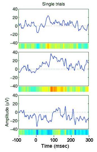
By stacking above each other the color-sequence lines for all trials in a dataset, we produce an ERP image:
Do ERPs arise through partial phase synchronization of the EEG?
In a ‘pure’ case of (partial) phase synchronization:
- EEG power (at the relevant frequencies) remains constant in the post-stimulus interval.
- The ITC value is significant during the ERP, but less than 1 (complete phase locking).
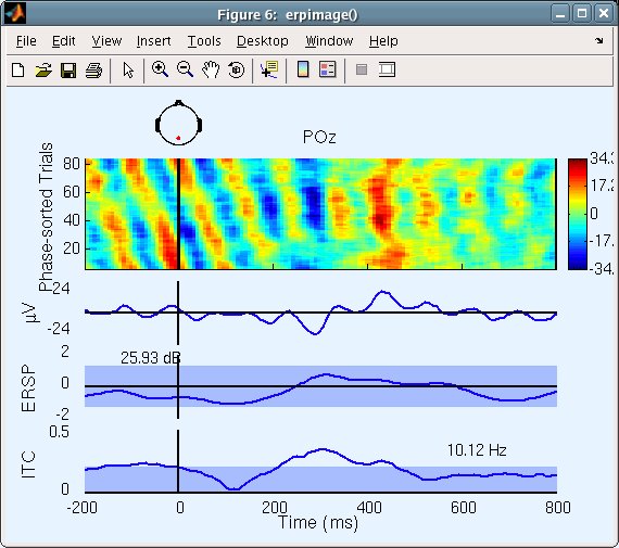
In our case, the figure (above) shows a significant post-stimulus increase in alpha ITC accompanied by a small (though non-significant) increase in alpha power. In general, an ERP could arise from partial phase synchronization of ongoing activity combined with a stimulus-related increase (or decrease) in EEG power.
It is important not to overinterpret the results of phase sorting in ERP-image plots. For example, the following calls from the MATLAB command line simulate 256 1-s data epochs using Gaussian white noise, low-pass filters this below (simulated) 12 Hz, and draw the following 10-Hz phase sorted ERP-image plot of the resulting data. The figure appears to identify temporally coherent 10-Hz activity in the (actual) noise. The (middle) amplitude panel below the ERP-image plot shows, however, that amplitude at (simulated) 10 Hz does not change significantly through the (simulated) epochs, and the lowest panel shows that inter-trial coherence is also nowhere significant (as confirmed visually by the straight diagonal 10-Hz wavefronts in the center of the ERP image).
% Simulate 256 1-s epochs with Gaussian noise
% at 256-Hz sampling rate; lowpass < 12 Hz
data = eegfilt(randn(1,256*256),256,0,15);

% Plot ERP image, phase sorted at 10 Hz
figure;
erpimage(data,zeros(1,256),1:256,'Phase-sorted Noise',1,1,...
 'phasesort',[128 0 10],'srate',256,...
 'coher',[10 10 .01], 'erp','caxis',0.9);
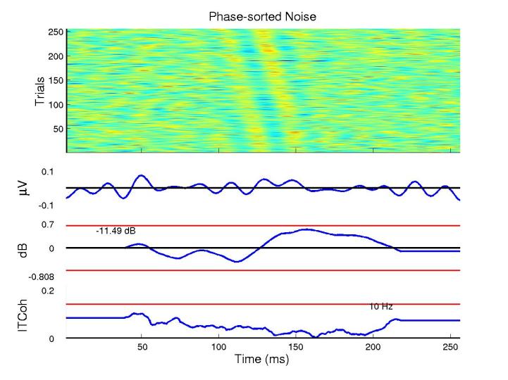
Taking epochs of white noise (as above) and adding a strictly time-locked ‘ERP-like’ transient to each trial will give a phase-sorted ERP-image plot showing a sigmoidal, not a straight diagonal wavefront signature. How can we differentiate between the two interpretations of the same data (random EEG plus ERP versus partially phase reset EEG)? For simulated one-channel data, there is no way to do so since both are equally valid ways of looking at the same (simulated) data - no matter how it was created. After all, the simulated data themselves do not retain any impression of how they were created - even if such an impression remains in the mind of the experimenter!
For real data, we must use convergent evidence to bias our interpretation towards one or the other (or both) interpretations. The partial phase resetting model begins with the concept that the physical sources of the EEG (partial synchronized local fields) may also be the sources of or contributors to average-ERP features. This supposition may be strengthened or weakened by examination of the spatial scalp distributions of the ERP features and of the EEG activity. However, here again, a simple test may not suffice since many cortical sources are likely to contribute to both EEG and averaged ERPs recorded at a single electrode (pair). An ERP feature may result from partial phase resetting of only one of the EEG sources, or it may have many contributions, including truly ‘ERP-like’ excursions with fixed latency and polarity across trials, monopolar ‘ERP-like’ excursions whose latency varies across trials, and/or partial phase resetting of many EEG processes. Detailed spatiotemporal modeling of the collection of single-trial data is required to parcel out these possibilities. For further discussion of the question in the context of an actual data set, see Makeig et al. (2002). In that paper, phase resetting at alpha and theta frequencies was indicated to be the predominant cause of the recorded ERP (at least at the indicated scalp site, POz). How does the ERP in the figure above differ?
The Makeig et al. (2002) paper dealt with non-target stimuli, whereas for the sample EEGLAB dataset, we used epochs time-locked to target stimuli from one subject (same experiment). The phase synchronization might be different for the two types of stimuli. Also, the analysis in the paper was carried out over 15 subjects and thousands of trials, whereas here, we analyze only 80 trials from one subject. (The sample data we show here are used for tutorial purposes. We are now preparing a full report on the target responses in these experiments.)