Analyzing EEG-BIDS data with EEGLAB scripts
Here we demonstrate how to import EEG-BIDS data into EEGLAB and use the EEGLAB STUDY tool for group analysis on these data to perform some basic EEGLAB group-level processing. You may also watch the series of short YouTube videos below. Click on the icon on the top right corner to access the list of videos in the playlist.
Table of contents
EEG-BIDS
The data in this tutorial are organized according to the EEG BIDS format. You can read more on the specificities of the EEG-BIDS format here. EEGLAB has a dedicated plugin called EEG-BIDS to export and import BIDS datasets. This plugin is available using the EEGLAB plugin manager and must be installed before running the scripts in this tutorial. It is worthwhile spending some time looking at how the files are organized in this BIDS example, as we will follow this convention throughout.
To know more about the integration of BIDS into EEGLAB, you can also visit the bids-matlab-io EEGLAB plugin documentation.
Download the data
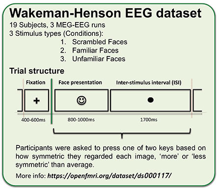
The EEG data used in this example comes from Wakeman and Henson (2015). In this experiment, simultaneous MEG-EEG data were collected while subjects viewed famous, unfamiliar, and scrambled faces. Each image was repeated three times, and subjects pressed one of two keys with their left or right index finger, indicating how symmetric they regarded each image relative to the average.
Human perception of suddenly presented face images produces a large negative peak at about 170 ms (dubbed ‘the N170’) in averaged event-related potentials (ERPs) for posterior scalp channels (Bentin et al., 1996). This potential has been localized by several methods, including direct electrocorticographic (ECoG) recording from the cortical surface, to the bilateral fusiform gyrus.
Henson and Wakeman (2015) apply joint EEG/MEG source analysis to the N170 peak scalp maps to estimate the areas of the inferior temporal cortex that produce the response feature. A BOLD signal increase in the same areas is seen in fMRI studies (Kanwisher et al., 1997). A long train of functional imaging and EEG experiments have considered the question of whether activation of fusiform gyrus by face image presentations indexes face-specific processing (Kanwisher & Yovel, 2006) or processing supporting more general expert identification of individuals or subcategories for any large set of important and long-studied objects – for example, automobile grilles by automobile experts (Gauthier et al., 1999).
Generally, face presentations produce much larger ‘N170’ potentials (and ensuing fusiform BOLD activations) than do presentations of ‘face-like’ images of houses, etc.
Wakeman and Henson (2015) developed the paradigm used to collect the data treated here to determine how repetition (of the same face image) in a series of tachistoscopically presented ‘face versus house’ images experiment affected EEG and concurrent MEG responses, and how responses to well-known, unknown, and scrambled faces in the same sequence differed. See details of the paradigm in the figure below.
The original dataset containing both EEG and MEG is quite large, so the raw data was transformed into a form that could be used for tutorials. The data were prepared (i.e., EEG extracted, timing corrected, electrode positions re-oriented, events latency corrected and renamed) by Dung Truong, Ramon Martinez & Arnaud Delorme and can be downloaded from OpenNeuro.
Data pre-processing
Once you have downloaded the data on OpenNeuro, you may run the code below (refer to this page if you experience problems downloading the data).
Start EEGLAB
In the scripts below, we use the git version of EEGLAB available as of 2021. Scripts may not work with earlier versions of EEGLAB.
clear
[ALLEEG, EEG, CURRENTSET, ALLCOM] = eeglab;
The code below assumes you have saved the data in the EEGLAB “sample_data” subfolder. If this is not the case, adjust the filepath variable in the cell below :
eeglabPath = fileparts(which('eeglab'));
filepath = fullfile(eeglabPath, 'sample_data', 'ds002718');
Import BIDS data
The function pop_importbids.m imports a BIDS format folder structure into an EEGLAB study. If ‘bidsevent’ is ‘on’ then events will be imported from the BIDS .tsv event file, and events in the raw binary EEG files will be ignored. Similarly, ‘bidschanloc’, ‘on’ will import channel locations from BIDS .tsv file and ignore any locations in raw EEG files. The ‘studyName’ field lets you specify the name of the newly created STUDY. See the BIDS import tutorial for more details on how to import BIDS studies.
[STUDY, ALLEEG] = pop_importbids(filepath, 'eventtype','trial_type', 'bidsevent','on','bidschanloc','on', ...
    'studyName','Face_detection');

ALLEEG = pop_select( ALLEEG, 'nochannel',{'EEG061','EEG062','EEG063','EEG064'}); % remove EKG and EOG
EEG=pop_chanedit(EEG, 'eval','chans = pop_chancenter( chans, [],[]);'); % center channels

CURRENTSTUDY = 1; EEG = ALLEEG; CURRENTSET = [1:length(EEG)];
We will perform artifact rejection in three steps:
- Mild artifact rejection using the clean_rawdata plugin
- Rejection of artifactual independent components
- Aggressive artifact rejection using the clean_rawdata plugin
We are using three steps for rejecting artifacts because there are large numbers of high-amplitude eye blinks in this data. Before running ICA, the data needs to be cleaned of major artifacts in step 1. If we had used the automated aggressive artifact rejection using the clean_rawdata plugin before running ICA, then all data portions containing blinks would have been removed. This is not desirable because ICA can remove/subtract blinks from the data. Then in step 3, once the data has been cleaned by ICA, other remaining artifacts may be removed using clean_rawdata.
Often, only steps 1 and 2 are necessary. This will depend on the data.
Remove bad channels and regions of activity with extreme artifacts
Here we are using the pop_clean_rawdata.m function to high-pass filter the data at 0.5 Hz, reject channels with abnormal activity, and remove data portions with extreme artifactual activity. The pop_clean_rawdata.m uses the Artefact Subspace Reconstruction (ASR) module that is integrated into the EEGLAB clean_rawdata() plugin (installed by default in EEGLAB).
EEG = pop_clean_rawdata( EEG,'FlatlineCriterion',5,'ChannelCriterion',0.8,...
    'LineNoiseCriterion',4,'Highpass',[0.25 0.75],'BurstCriterion',40,...
    'WindowCriterion',0.25,'BurstRejection','on','Distance','Euclidian',...
    'WindowCriterionTolerances',[-Inf 10] );
Re-reference using the average reference
Average reference may be applied multiple times during processing. Applying average reference at a given time cancels all re-referencing done before that time. This is not a required step.
EEG = pop_reref( EEG,[],'interpchan',[]);
Run ICA and flag artefactual components using IClabel
Then, we apply ICA to the data. If you have installed the Picard plugin for EEGLAB, you may replace ‘runica’ by ‘picard’. As ‘runica’, Picard is an Infomax ICA algorithm but uses the newton optimization method, which is both faster and theoretically more efficient. You can find more details on using ICA to remove artifacts embedded in EEG data by reading the dedicated section on the EEGLAB tutorial.
Then we use IClabel to classify components. IClabel is an EEGLAB plugin installed by default with EEGLAB, which calculates a probability for the type of each independent component (brain, eye, muscle, line noise, etc.). Note that the second argument of the function pop_icflag.m ‘thresh’ is to specify the minimum and maximum threshold values used for selecting components as artifacts. The thresholds are entered for 6 categories of ICA components that are, in order: Brain, Muscle, Eye, Heart, Line Noise, Channel Noise, Other. So here, you can see that we only remove ICA components if they are classified in the Eye or Muscle with at least 80% confidence. ICA components that are flagged as artefactual by IClabel are then subtracted (removed) from the data.
EEG = pop_runica(EEG, 'icatype','runica','concatcond','on',...
                                'options',{'pca', -1});
EEG = pop_iclabel(EEG,'default');
EEG = pop_icflag(EEG,[NaN NaN;0.8 1;0.8 1;NaN NaN;NaN NaN;NaN NaN;NaN NaN]);
EEG = pop_subcomp(EEG, [], 0, 0); %remove bad components
Remove remaining portions of contaminated data
Again we are using ASR and pop_clean_rawdata.m here, but this time to aggressively remove portions of data containing remaining artefactual activity. First, ASR finds clean portions of data (calibration data) and calculates the standard deviation of PCA-extracted components (ignoring physiological EEG alpha and theta waves by filtering them out). Then, it rejects data regions if they exceed 20 times (by default) the standard deviation of the calibration data. The lower this threshold, the more aggressive the rejection is.
EEG = pop_clean_rawdata( EEG,'FlatlineCriterion','off','ChannelCriterion','off',...
    'LineNoiseCriterion','off','Highpass','off','BurstCriterion',20,...
    'WindowCriterion',0.25,'BurstRejection','on','Distance','Euclidian',...
    'WindowCriterionTolerances',[-Inf 7] );
Note that dataset 15 (EEG(15)) only has 15% data left at the end of this process and that the threshold above are likely too aggressive. You can access the description of each of this function’s parameter from within MATLAB by typing:
help pop_clean_rawdata
Extract data epochs
Below, we convert the continuous EEG datasets to epoched datasets by extracting data epochs that are time-locked to the specified event types. The ‘timelim’ input defines the epoch latency limits in seconds relative to the time-locking events: here, we define a window from -0.5s before the event to 1s after the event. Note that we do not remove a baseline (high-pass filtering performed above is sufficient at this stage).
EEG = pop_epoch( EEG,{'famous_new','famous_second_early','famous_second_late','scrambled_new','scrambled_second_early','scrambled_second_late','unfamiliar_new','unfamiliar_second_early','unfamiliar_second_late'},[-0.5 1] ,'epochinfo','yes');
Data plotting
Creating a STUDY design
The code below will create a STUDY design to compare across conditions.
ALLEEG = EEG; % update ALLEEG structure
STUDY = std_checkset(STUDY, ALLEEG); % update epoch information
STUDY = std_makedesign(STUDY, ALLEEG, 1, 'name','Faces','delfiles','off','defaultdesign','off',...
    'variable1','face_type','values1',{'famous','scrambled','unfamiliar'},...
    'vartype1','categorical', ...
    'subjselect',{'sub-002','sub-003','sub-004','sub-005','sub-006','sub-007','sub-008','sub-009',...
    'sub-010', 'sub-011','sub-012','sub-013','sub-014','sub-015','sub-016','sub-017','sub-018','sub-019'});
Update the main EEGLAB window.
eeglab redraw
Compute channels measures
Note that this can be done before creating a study design. Here, we compute event-related potentials. This is computed over each individual channel. Below, we only per-compute ERPs, with a -200 ms to 0 ms baseline.
[STUDY, ALLEEG] = std_precomp(STUDY, ALLEEG, {},'savetrials','on','rmicacomps','on','interp','on',...
    'recompute','on','erp','on','erpparams',{'rmbase',[-200 0] });
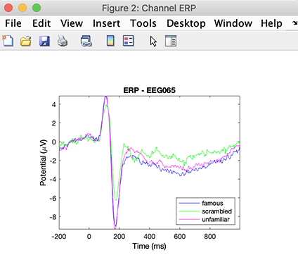
Plot ERP at a single channel
Now we are going to plot the ERPs for one channel for each of the conditions. We first specify plotting parameters.
STUDY = pop_erpparams(STUDY, 'timerange',[-200 1500], 'plotconditions','together');
Then we plot the figure (here, we select channel 65 as in the original publication).
STUDY = std_erpplot(STUDY,ALLEEG,'channels',{'EEG065'}, 'design', 1);
More details about plotting STUDY measure is available in the STUDY visualization tutorial.
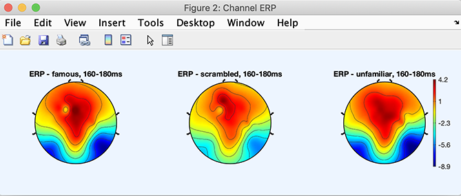
Plot the ERP activity as an averaged topographical map
We first change the plotting parameters to plot the scalp topography 170 ms after stimulus presentation (average of the potential between 160 and 180 ms).
STUDY = pop_erpparams(STUDY, 'topotime',[160 180] ,'timerange',[]);
and then, we plot the scalp topography.
STUDY = std_erpplot(STUDY,ALLEEG,'channels',{'EEG001','EEG002','EEG003','EEG004', ...
'EEG005','EEG006', 'EEG007','EEG008','EEG009','EEG010','EEG011','EEG012','EEG013', ...
'EEG014','EEG015','EEG016','EEG017','EEG018','EEG019','EEG020','EEG021','EEG022','EEG023','EEG024', ...
'EEG025','EEG026','EEG027','EEG028','EEG029','EEG030','EEG031','EEG032','EEG033','EEG034','EEG035', ...
'EEG036','EEG037','EEG038','EEG039','EEG040','EEG041','EEG042','EEG043','EEG044','EEG045','EEG046', ...
'EEG047','EEG048','EEG049','EEG050','EEG051','EEG052','EEG053','EEG054','EEG055','EEG056','EEG057', ...
'EEG058','EEG059','EEG060','EEG065','EEG066','EEG067','EEG068','EEG069','EEG070','EEG071', ...
'EEG072','EEG073','EEG074'}, 'design', 1);
This tutorial was a simple demonstration of how to process BIDS data. At this point, you may refer to the group analysis tutorial to perform statistics or advanced processing of brain source activities on this data. You may also look at the LIMO plugin tutorial, which uses the same BIDS data to perform statistical analyses based on the general linear model.