Independent Component Analysis for artifact removal

Independent Component Analysis (ICA) may be used to remove/subtract artifacts embedded in the data (muscle, eye blinks, or eye movements) without removing the affected data portions. ICA may also be used to find brain sources, and we will come back to this topic in subsequent sections of the tutorial. For more theory and background information on ICA you can also refer to the Appendix.

Watch ICA presentations

You may watch below eleven short presentations on EEG independent component analysis (part of the EEGLAB online tutorial). If you click on the icon on the top right corner, you can see the list of all the videos in the playlist.

Running ICA decompositions

Load the sample EEGLAB dataset

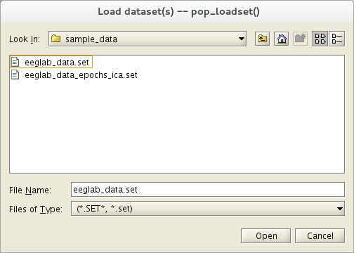
Select menu item File and press sub-menu item Load existing dataset. Select the tutorial file “eeglab_data.set” located in the “sample_data” folder of EEGLAB. Then press Open.

In theory, you should go through rejecting bad channels and bad portions of data before running ICA. However, the tutorial dataset is clean enough for running ICA without prior artifact rejection.

This dataset already contains channel locations. However, when working with a dataset that does not have channel locations, select the Edit → Channel locations menu item and press Ok to look up channel locations based on channel labels, then close the channel editor.

Run ICA

To compute ICA components of a dataset of EEG epochs (or of a continuous EEGLAB dataset), select Tools → Decompose data by ICA. This calls the function pop_runica.m. To run ICA using the default options, simply press Ok.

We detail each entry of this GUI in detail below.

Which ICA Algorithm?

EEGLAB allows users to try different ICA decomposition algorithms. Infomax ICA using runica.m, Jader algorithm using jader.m, and the SOBI algorithm using the sobi.m are all part of the default EEGLAB distribution. Other options available in the dropdown list of algorithms are a modified version of SOBI for data epochs (acsobiro.m), and binica.m which is a compiled C-version of Infomax (as opposed to the MATLAB runica.m version).

To use the FastICA algorithm, one must install the FastICA toolbox and include it in the MATLAB path. You may also install the ICALAB distribution, which contains other algorithms, or install the Picard EEGLAB plugin, a version of Infomax implementing Newton optimization. ICA algorithms installed with these tools will automatically appear in the dropdown list of available ICA algorithms in the previous section’s graphic interface.

You may install the Amica and postAmicaUtility plugins to use Amica in EEGLAB. By contrast with other ICA algorithms, Amica does not use the standard ICA interface and creates its own sets of menus.

Refer to the ICA concept guide for further information on the different ICA algorithms.

Important note

We usually run ICA using many more trials than the sample decomposition presented here. ICA works best when given a large amount of basically similar and mostly clean data. When the number of channels (N) is large (>>32), then a considerable amount of data may be required to find N components. When insufficient data are available, then use the ‘pca’ option to find fewer than N components may be the only good option. In general, it is important to give ICA as much data as possible for successful training. Refer to the ICA concept guide for more details.

Selecting channel types

It is possible to select specific channel types (or even a list of channel numbers) to use for ICA decomposition. For instance, if you have both EEG and EMG channels, you may want to run ICA on EEG channels only since any relationship between EEG and EMG signals should involve propagation delays. ICA assumes an instantaneous relationship (e.g., common volume conduction). Use menu item Edit → Channel locations to define channel types.

Command-line output

Running runica.m produces the following text on the MATLAB command line:

    Input data size [32,30720] = 32 channels, 30720 frames.
    Finding 32 ICA components using logistic ICA.
    Initial learning rate will be 0.001, block size 36.
    Learning rate will be multiplied by 0.9 whenever angledelta >= 60 deg.
    Training will end when wchange < 1e-06 or after 512 steps.
    Online bias adjustment will be used.
    Removing mean of each channel ...
    Final training data range: -145.3 to 309.344
    Computing the sphering matrix...
    Starting weights are the identity matrix ...
    Sphering the data ...
    Beginning ICA training ...
    step 1 - lrate 0.001000, wchange 1.105647
    step 2 - lrate 0.001000, wchange 0.670896
    step 3 - lrate 0.001000, wchange 0.385967, angledelta 66.5 deg
    step 4 - lrate 0.000900, wchange 0.352572, angledelta 92.0 deg
    step 5 - lrate 0.000810, wchange 0.253948, angledelta 95.8 deg
    step 6 - lrate 0.000729, wchange 0.239778, angledelta 96.8 deg
    ...
    step 55 - lrate 0.000005, wchange 0.000001, angledelta 65.4 deg
    step 56 - lrate 0.000004, wchange 0.000001, angledelta 63.1 deg
    Inverting negative activations: 1 -2 -3 4 -5 6 7 8 9 10 -11 -12 -13 -14 -15 -16 17 -18 -19 -20 -21 -22 -23 24 -25 -26 -27 -28 -29 -30 31 -32
    Sorting components in descending order of mean projected variance ...
    1 2 3 4 5 6 7 8 9 10 11 12 13 14 15 16 17 18 19 20 21 22 23 24 25 26 27 28 29 30 31 32

Note: The Infomax algorithm implemented in runica.m can only select for components with a super-gaussian activity distribution (i.e., more highly peaked than a Gaussian, something like an inverted T). If there is strong line noise in the data, use the option ‘’ ‘extended’, 1’’ in the command-line edit box (set as default), so the algorithm can also detect subgaussian sources of activity, such as line current and/or slow activity.

Another option we often use is the stop option: try ‘’ ‘stop’, 1E-7’’ to lower the criterion for stopping learning, thereby lengthening ICA training but possibly returning cleaner decompositions, particularly of high-density array data.

Important note: Run twice on the same data, ICA decompositions under runica.m will differ slightly. That is, the ordering, scalp topography, and activity time courses of best-matching components may appear slightly different. This is because ICA decomposition starts with a random weight matrix (and randomly shuffles the data order in each training step), so the convergence is slightly different every time. Is this a problem? At the least, the decomposition features that do not remain stable across decompositions of the same data should not be interpreted except as irresolvable ICA uncertainty. The RELICA plugin allows assessing the reliability of ICA decomposition when bootstrapping the data.

Differences between decompositions trained on somewhat different data subsets may have several causes. We have not yet performed such repeated decompositions and assessed their common features - though this would seem a sound approach.

For this tutorial, we decide to accept the initial ICA decomposition of our data and study its independent components’ nature and behavior(s).

First, we review a series of functions whose purpose is to determine which components to study and how to study them.

Inspecting ICA components

The component order returned by runica.m is in decreasing order of the EEG variance accounted for by each component. In other words, the lower the order of a component, the more data (neural and/or artifactual) it accounts for.

Scrolling through component activations

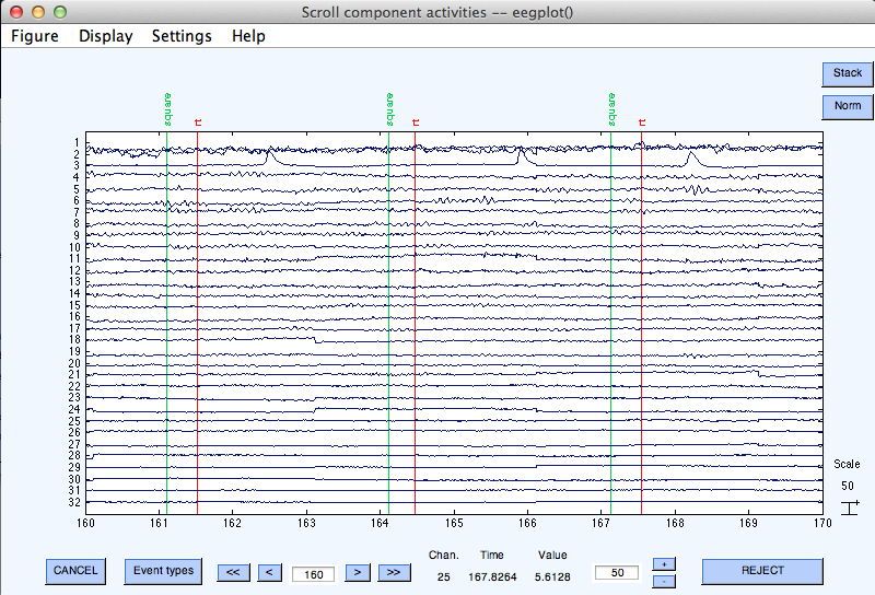
To scroll through component activations (time courses), select Plot → Component activations (scroll). Scrolling through the ICA activations, one may easily spot components accounting for characteristic artifacts. For example, in the scrolling eegplot.m below, component 3 appears to account primarily for blinks (we will learn how to recognize components in this tutorial).

Plotting 2-D Component Scalp Maps

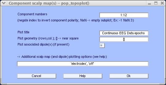
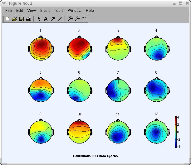
To plot 2-D scalp component maps, select Plot → Component maps → In 2-D. The interactive window (below) is then produced by function pop_topoplot.m. Simply press Ok to plot all components.

Note: This may take several figures, depending on the number of channels and the Plot geometry parameter. An alternative is to call this function several times for smaller groups of channels (e.g., 1:30 , 31:60 , etc.). Below we ask for the first 12 components (1:12) only, and choosing to set ‘electrodes’, ‘off’.

The following topoplot.m window appears, showing the scalp map projection of the selected components. Note that the scale in the following plot uses arbitrary units. The scale of the component’s activity time course also uses arbitrary units. However, the component’s scalp map values multiplied by the component activity time course are in the same unit as the data.

Studying and flagging artifactual ICA components

Learning to recognize types of independent components may require experience. A later section on Automated detection of artifactual ICA components on this page contains links to an online tutorial for learning to recognize components.

The main criteria to determine if a component is 1) cognitively related 2) a muscle artifact, or 3) some other type of artifacts are

• First, the scalp map (as shown above),
• Next the component time course,
• Next the component activity power spectrum,
• Finally (given a dataset of event-related data epochs), the erpimage.m.

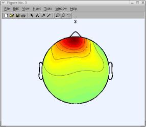
In the window above, click on scalp map number 3 to pop up a window showing it alone (as mentioned earlier, your decomposition and component ordering might be slightly different). An expert eye would spot component 3 (below) as an eye artifact component.

To study component properties and label components for rejection (i.e., to identify components to subtract from the data), select Tools → Inspect/label components by maps.

The difference between the resulting figure(s) and the previous 2-D scalp map plots is that one can here plot each component’s properties by clicking on the rectangular button above each component scalp map.

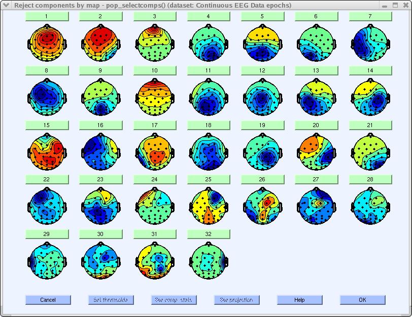
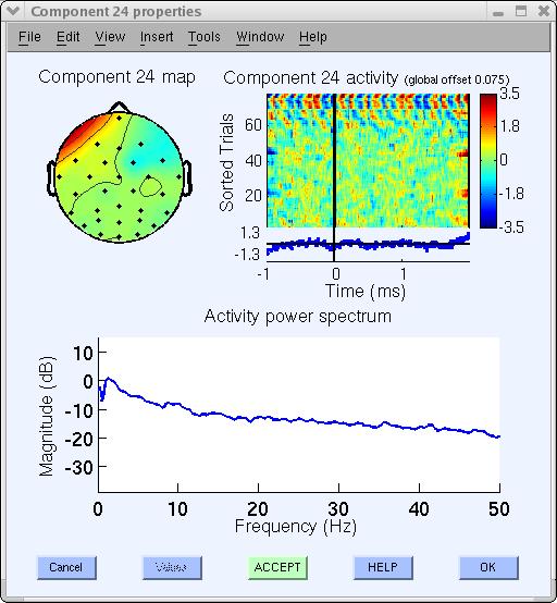
For example, click on the button labeled 3. This component can be identified as an eye artifact for three reasons:

1. The smoothly decreasing EEG spectrum (bottom panel) is typical of an eye artifact;
2. The scalp map shows a strong far-frontal projection typical of eye artifacts; And,
3. It is possible to see individual eye movements in the component erpimage.m (top-right panel).

Eye artifacts are (nearly) always present in EEG datasets. They are usually in leading positions in the component array (because they tend to be big) and their scalp topographies (if accounting for lateral eye movements) look like component 3 or perhaps (if accounting for eye blinks) like that of component 10 (above).

You can also access component property figures directly by selecting Plot → Component properties. (There is an equivalent menu item for channels, Plot → Channel properties).

Artifactual components are also relatively easy to identify by visual inspection of component time course (menu Plot → Component activations (scroll) — not shown here).

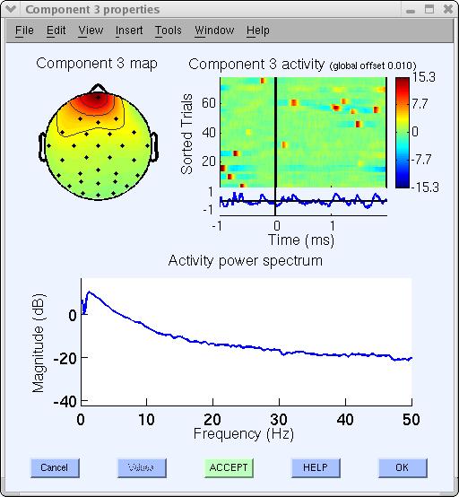
Since this component accounts for eye activity, we may wish to subtract it from the data before further analysis and plotting. If so, click on the bottom green Accept button (above) to toggle it into a red Reject button (note: at this point, components are only marked for rejection; to subtract marked components, see the section of this page on Subtracting ICA components from data. Now press Ok to go back to the main component property window.

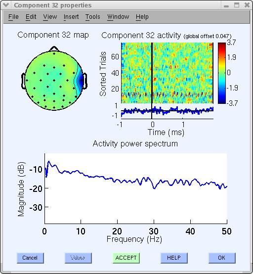
Another artifact example in our decomposition is component 32, which appears to be a typical muscle artifact component. This component is spatially localized and shows high power at high frequencies (20-50 Hz and above), as shown below.

Artifactual components often encountered (but not present in this decomposition) are single-channel (channel-pop) artifacts in which a single channel goes ‘off,’ or line-noise artifacts such as 23. The ERP image plot below shows that it picked up some line noise at 60 Hz, especially in trials 65 and on.

Many other components appear to be brain-related. A different section of the tutorial deals with using ICA component for brain source localization. What if a component looks to be “half artifact, half brain-related”? In this case, we may ignore component 23, or may try running ICA decomposition again on a cleaner data subset or using other ICA training parameters.

As a rule of thumb, we have learned that removing artifactual data regions containing one-of-a-kind artifacts is very useful for obtaining ‘clean’ ICA components.

Optimizing ICA decompositions’ quality

What do we mean by obtaining a better ICA decomposition?

ICA takes all training data into consideration. When too many types (i.e., scalp distributions) of noise - complex movement artifacts, electrode pops, etc – are left in the training data, these unique and irreplicable data features will draw the attention of ICA, producing a set of component maps including many single-channel or noisy-appearing components. The number of components (degrees of freedom) devoted to the decomposition of brain EEG alone will be correspondingly reduced.

Therefore, presenting ICA with as much clean EEG data as possible is the best strategy. Note that blink and other stereotyped EEG artifacts do not necessarily have to be removed since they are likely to be isolated as single ICA components.

Here clean EEG data means data after removing noisy time segments (does not apply to removed ICA components).

How to deal with the aggressive high-pass filter applied before running ICA

ICA decompositions are notably higher quality (less ambiguous components) when the data is high-pass filtered above 1 Hz or sometimes even 2 Hz. High-pass filtering is the easiest solution to fix bad quality ICA decompositions. However, for processing EEG data (such as ERP analysis), high-pass filtering at 2 Hz might not be optimal as it might remove essential data features. In this case, we believe an optimal strategy is to:

1. Start with an unfiltered (or minimally filtered) dataset (dataset 1)
2. Filter the data at 1Hz or 2Hz to obtain dataset 2
3. Run ICA on dataset 2
4. Apply the resulting ICA weights to dataset 1. To copy ICA weights and sphere information from dataset 1 to 2: First, call the Edit → Dataset info menu item for dataset 1. Then enter ALLEEG(2).icaweights in the ICA weight array … edit box, ALLEEG(2).icasphere in the ICA sphere array … edit box, and press Ok.

ICA components can be considered as spatial filters, and it is perfectly valid to use these spatial filters on the original unfiltered data. The only limitation is that since strong artifacts affect low-frequency bands filtered out before using ICA, they may not be removed by ICA. In practice, we have never found this to be a problem because artifactual processes that contaminate the data below 2 Hz also tend to contaminate the data above 2 Hz.

What to do with a low-quality ICA decomposition

With a low-quality ICA decomposition, you can try filtering the data as indicated in the previous section. Another strategy is to clean the data aggreesively of artifacts before running ICA as explained below:

1. Start with an unfiltered (or minimally filtered) dataset (dataset 1)
2. Aggressively clean dataset either manually or using the automated tools provided in EEGLAB to obtain dataset 2
3. Run ICA on dataset 2
4. Apply the resulting ICA weights to dataset 1. To copy ICA weights and sphere information from dataset 1 to 2: First, call the Edit → Dataset info menu item for dataset 1. Then enter ALLEEG(2).icaweights in the ICA weight array … edit box, ALLEEG(2).icasphere in the ICA sphere array … edit box, and press Ok.

As mentioned previously, ICA components can be considered as spatial filters, and it is perfectly valid to use these spatial filters on the original unfiltered data. One limitation of this approach is that the quality of ICA decompositions depends on the quantity of EEG data provided as input. Reducing the amount of data could decrease the overall quality of an ICA decomposition.

How to deal with corrupted ICA decompositions

When using Infomax ICA, which is the default in EEGLAB, the first two components’ activity can blow up. This happens because the two components’ activities compensate for each other. Both components are almost identical with opposite polarities. In this case, both components are seen as having a large amount of noise. This is illustrated below.

This may happen in case of rank deficiency (as explained in the next section). However, this may also happen in full ranked data. The solution to this problem is not obvious. One solution is to use a different ICA algorithm. Another solution is to experiment with decreasing the number of dimensions using PCA. For example, with 32 channels, decreasing the number of dimensions to 10 could eliminate the problem (decreasing to 20 did not). Below is the same data but decomposed with only 10 PCA components (only the first component is shown). Not only does this component account for both component activities above, but the noise in its activation disappears (i.e., is more properly assigned by ICA to other component processes). The noise above is most likely due to instability in the ICA decomposition algorithm, which here forced to create two components compensating for each others’ activity. We are not sure that removing the single blink component below is preferable to removing the two very noisy components above since we have not run any formal comparison. Our reasoning is that the two components above tend to make other components noisy, so the PCA dimension reduction solution is preferable.

This is not to say that using PCA should be done systematically. In general, PCA will slightly corrupt the data by adding nonlinearities, so it is better to use the full rank data matrix whenever possible.

A full discussion of corrupted ICA components, also called Ghost ICA components, is available in this paper and this one.

Issues with data rank deficiencies

When computing average reference on n-channel data, the rank of the data is reduced to n-1. Why? Because the sum of the potential is 0 at all time points, the last channel activity is equal to minus the sum of the others. ICA does not behave well in this (rank-deficient) case.

If the rank of the data is lower than the number of channels, the EEGLAB pop_runica() function should detect it and uses different strategies to do so.

However, rank calculations in MATLAB are imprecise, especially since raw EEG data is stored as a single-precision matrix. Thus, there are some cases in which the rank reduction arising from using average reference is not detected. In this case, the user should manually reduce the number of components. If the ICA decomposition does not look “right” (with the types of components shown on this page), check on the MATLAB command line that EEGLAB reduced the number of dimensions. If this is not the case, you can fix this manually.

For example, when using 64 channels, enter “‘pca’, 63” in the option edit box. If you do not do this, the activity of one of the components that contributes the most to the data might be duplicated (as explained in the previous section), and you will not be able to use the ICA decomposition. Note that because of small numerical innacuracies inherent to digital signal processing, we recommend people compute ICA, then compute average reference after ICA (see this paper).

Issues associated with aggressive automated artifact removal before ICA

Automated artifact removal before ICA may remove data (such data portions containing blinks), which can easily be corrected by ICA. However, lowering the thresholds for automated artifact rejection might retain too many artifacts that ICA cannot remove. In this case, we recommend the following procedure.

1. Start with a dataset that has been minimally cleaned of artifacts (or where only bad channels have been removed)
2. Run ICA on this dataset
3. Identify bad ICA components and remove/subtract them from the data as explained in one of the following sections
4. Clean again the dataset using a more aggressive threshold or strategy to remove the remaining artifactual portions of data

Applying ICA to data epochs instead of continuous data

In general, we recommend using ICA on continuous data, not data for which epochs have been extracted. First, extracting data epochs reduces the number of samples, and ICA component quality is usually higher when more data is present. Second, you are not tempted to remove the epochs’ baseline. Removing the epoch baseline can have dramatic consequences for ICA because it introduces random offsets in each channel, something ICA cannot model or compensate for. Note that it is possible to extract epochs and not remove the epoch baseline. Then after running ICA, the baseline may be removed.

However, applying ICA to data epochs is possible. ICA expects the data to be stationary, i.e., the same statistical model is generating all data samples. If you have enough data after epoching, then epoched data might be preferable since it will be more stationary. However, when epoching on different events to produce different datasets, we recommend using the same ICA decomposition for all conditions. Practically, this may mean creating a dataset containing all epoch types before running ICA. More data generally gives a better ICA decomposition, assuming all the data is similar statistically. Longer epochs are preferable because they yield more data for ICA (assuming stationarity holds.)

However, if you are epoching before ICA,you don’t want to give ICA overlapping epochs since it will duplicate some data skewing the statistical model. For example, the pre-stimulus baseline portion of an epoch time-locked to a target stimulus may contain some portion of an epoch time-locked to a preceding nontarget stimulus event. Infomax ICA performed by pop_runica.m does not consider the time order of the data samples but selects time samples in random order during training. Thus, replicated data samples in concatenated datasets will only tend to be used more often during training. So the epoch start time should not be before the stop time of the previous epoch, and the stop time should not be after the start time of the next epoch.

Automated detection of artifactual ICA components

The ICLabel plugin of Luca Pion-Tonachini is an EEGLAB plugin installed by default with EEGLAB, which provides an estimation of the type of each of the independent components (brain, eye, muscle, line noise, etc.). The ICLabel project’s goal was to develop an EEG IC classifier that is reliable and accurate enough to use in large-scale studies. The current classifier implementation is trained on thousands of manually labeled ICs and hundreds of thousands of unlabeled ICs. More information may be found in the ICLabel reference article. The ICLabel website also allows you to train to recognize components and compare your performance with experts. Note that ICLabel is one of many such EEGLAB plugins that can automatically find artifactual ICA components. Other plugins or toolboxes worth checking for automatically labeling ICA components are MARA, FASTER, SASICA, ADUST, and IC_MARK.

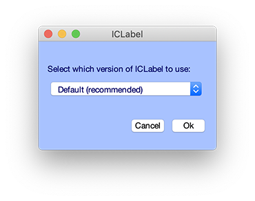
Once you have run ICA, select menu item Tools → Classify components using ICLabel → Label components. Simply select the default and press OK.

A second window will pop up and ask to plot components. Simply press Ok.

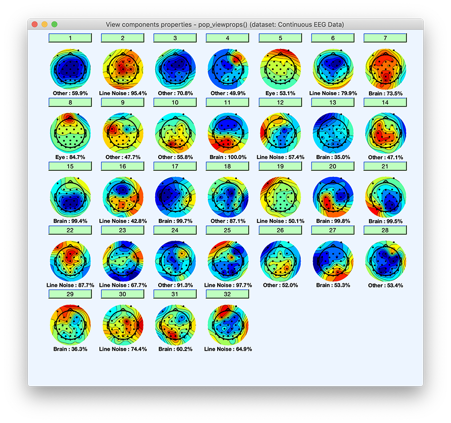
Clicking on a component will pop up a window with an expanded set of component property measures, as well as the estimated probabilities of each component being of each type. IC components will be plotted along with the category they most likely belong to and the likelihood of belonging to that category. Press Ok when done.

Note that the probability that a component belongs to a given category is also available on the MATLAB command line. There are six categories of components Brain, Muscle, Eye, Heart, Line Noise, Channel Noise, and Other. By typing the following command on the MATLAB prompt, you can see the probability for each of the first ten components (rows) to belong to one of the component categories (columns):

>>  round(EEG.etc.ic_classification.ICLabel.classifications(1:10,:)*100)

ans =

  10×7 single matrix

    12     0     1     0    26     1    60
     4     0     0     0    95     0     0
    10     0     4     0    14     1    71
    20     0     0     1    28     1    50
     9     0    53     2     9     2    26
     5     0     0     1    80     0    14
    74     0     0     0    12     0    14
     1     0    85     0     8     2     4
     7     0     0     0    41     4    48
    23     0     0     0    21     0    56

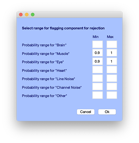
Then you may select menu item Tools → Classify components using ICLabel → Flag components as artifacts. The default is to label those components which have more than 90% probability of being in the muscle or eye artifacts (eye blinks and eye movements) category. When components are flagged using this function, the button will appear red in the interface for rejecting components manually (Tools → Reject using ICA → Reject components by map), so may edit which components have been flagged as artifacts.

Subtracting ICA components from data

Typically we do not subtract whole independent component processes from our datasets because we study individual component (rather than summed scalp channel) activities. Also, even you are only interested in removing ICA components, at the STUDY level (group analysis level), components you have flagged as artifacts, either manually or using an automated method, may be automatically subtracted from the data. Therefore, there is no need to physically remove/subtract components from the EEG data.

However, if we want to remove components, we use the Tools → Remove components menu item, which calls the pop_subcomp.m function.

The component numbers included by default in the resulting window (below) are those marked for rejection in the previous Tools → Reject using ICA → Reject components by map component rejection window (using the Accept or Reject buttons).

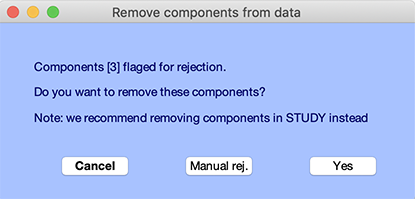
You may press Yes or select the Manual rej button to manually edit the list of components, as shown below.

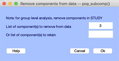
Enter the component numbers you wish to reject (in this case, we will leave component 3) and press Ok. Note that component 3 might not be an eye blink artifact in your case. Since your ICA decomposition might be slightly different, you will need to select manually (or using the automated detection of artifactual ICA components) the corresponding component. A window will pop up, asking if you want to compare the data before and after rejecting components, as shown below.

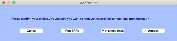
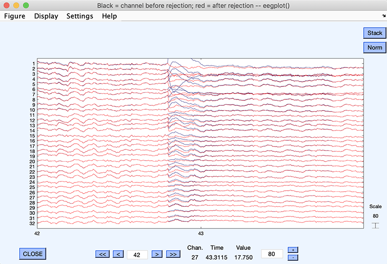
Click on Plot single trial pushbutton. This shows (below) the data before (in black) and after (in red) component(s) subtraction. We can clearly see how well ICA has removed the blink artifact.

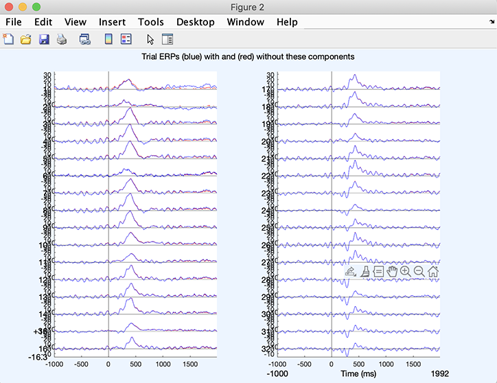
In case you are removing ICA component in data epochs, you may click on Plot ERPs pushbutton – it is possible to run ICA, extract epochs, and then remove ICA components. We have used continuous data for this tutorial, so we cannot plot ERPs. If we had extracted ERPs, we would obtain a plot similar to the one below, plotting channel ERP before (in blue) and after (in red) component(s) subtraction.

Once you are satisfied with the result, press the Accept button in the query window. Another window will pop up asking you if you want to rename the new data set. Give it a name and again press Ok.

In the rest of this tutorial, after running ICA, we pursue with retaining all components, so you can appreciate the contribution of artifactual components to ERPs.