Lets’ consider now all 9 conditions: 3 types of faces (familiar, unfamiliar, scrambled) and 3 repetition levels (immediate, small delay, long delay). This is analysed using a repeated measure ANOVA.

1st level analysis

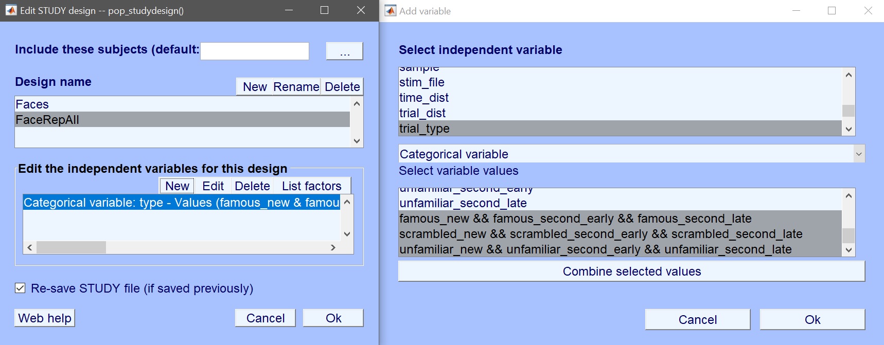
We need to compute a model for each subject, in which all 9 conditions are present. This should have been done already if you have computed the 1st level for the 1-way ANOVA revised section – if not, do it as proposed, i.e. setting up the model with contrasts (figure 20).

2nd level analysis

We can now compute the repeated measure ANOVA at the group level, using beta files. The model is a repeated measure ANOVA with 1 group, and 2 factors of three levels i.e. [3 3]. As you will notice, the computational time is higher, since now we have 2 additional effects to compute, not just the face effect but also the repetition effect and the interaction. Each one can be visualized using image all in the result GUI (figure 32 for ERP, Spectrum and ERSP ).

Figure 32a. 2*2 ANOVA ERP
Figure 32b. 2*2 ANOVASpectrum
Figure 32c. 2*2 ANOVA ERSP
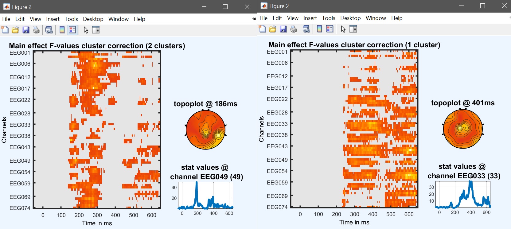
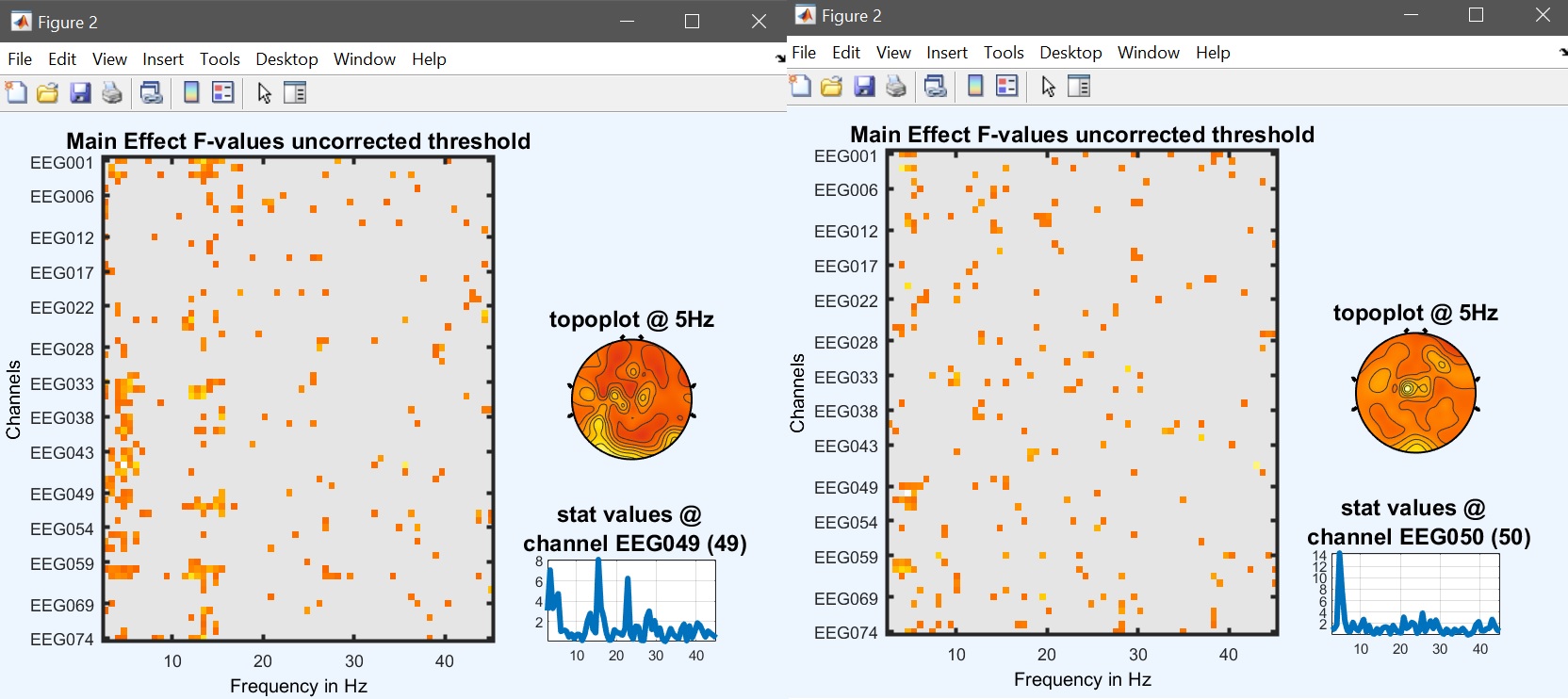
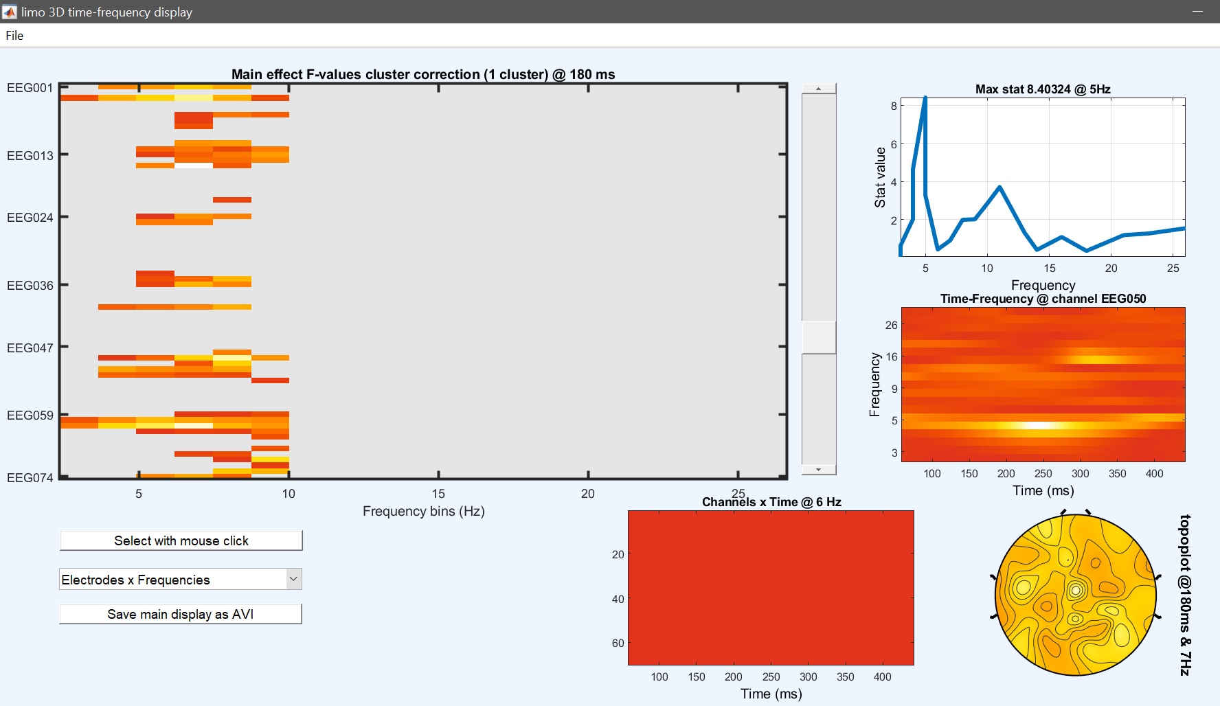
Figure 32. Main face effect (left) and repetition effect (right)

As with the one-way ANOVA, this analysis can be done in command line, here concatenating parameters into cell arrays.

cd(STUDY.filepath)
chanlocs = [STUDY.filepath filesep 'limo_gp_level_chanlocs.mat'];
mkdir('Face-Repetition_ANOVA');cd('Face-Repetition_ANOVA')
LIMOPath = limo_random_select('Repeated Measures ANOVA',chanlocs,'LIMOfiles',...
    fullfile(STUDY.filepath,['LIMO_' STUDY.filename(1:end-6)],'Beta_files_FaceRepAll_GLM_Channels_Time_WLS.txt'),...
    'analysis_type','Full scalp analysis','parameters',{[1 2 3],[4 5 6],[7 8 9]},...
    'factor names',{'face','repetition'},'type','Channels','nboot',1000,'tfce',0,'skip design check','yes');

Contrast

At this stage, as we did before we can perform some contrast to check which conditions are driving the effects. Let’s have a look at the difference Famous vs Unfamiliar – the contrast is [1 1 1 0 0 0 -1 -1 -1] (figure 33 for ERP, Spectrum and ERSP and compare that with a paired t-test (next section).

Figure 33a. Con ANOVA ERP
Figure 33b. Con ANOVASpectrum
Figure 33c. Con ANOVA ERSP
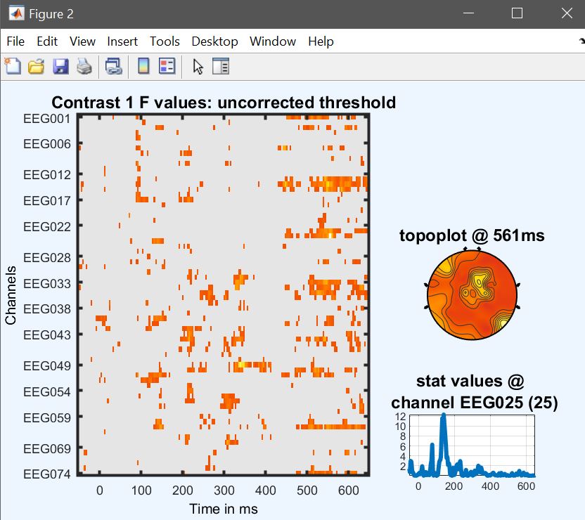
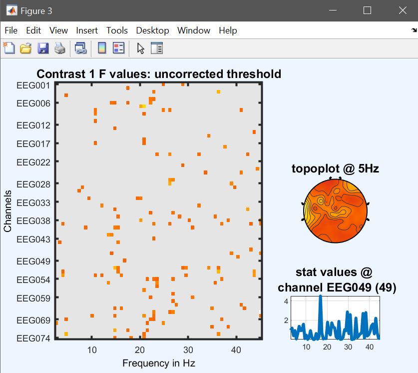
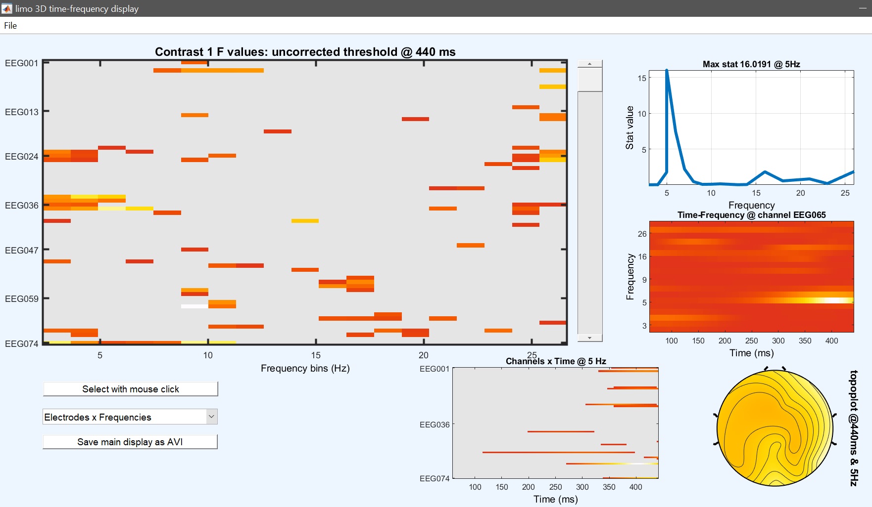
Figure 33. Contrast famous vs unfamiliar

% add contrast famous>unfamiliar
limo_contrast(fullfile(pwd,'Yr.mat'),fullfile(pwd,'LIMO.mat'), 3 ,[1 1 1 0 0 0 -1 -1 -1]); % compute a new contrast
limo_contrast(fullfile(pwd,'Yr.mat'),fullfile(pwd,'LIMO.mat'), 4);                         % do the bootstrap - although here there is no effect anyway