Removing bad channels by visual inspection

Bad channels are common when collecting EEG data. For example, this may be due to a bad connection. You may know in advance which channels are bad, or you may need to look at the data.

Load a sample EEGLAB dataset

The tutorial datasets distributed with EEGLAB are relatively clean and do not contain channels we normally reject. Instead, please download this other data file.

Select menu item File and press sub-menu item Load existing dataset. Select the tutorial file “eeglab_data_bad_channels.set” downloaded above. Then press Open.

Inspect data

Scrolling channel data

The next section contains extensive details on the data scrolling interface. Here, we will simply use it to visually identify bad channels. To scroll through the channel data of the current dataset, select Plot → Channel data (scroll). This pops up the scrolling data display window below. The window has been magnified vertically, so channel indices may be visible.

Image:scroll_data_bad_chan3.png

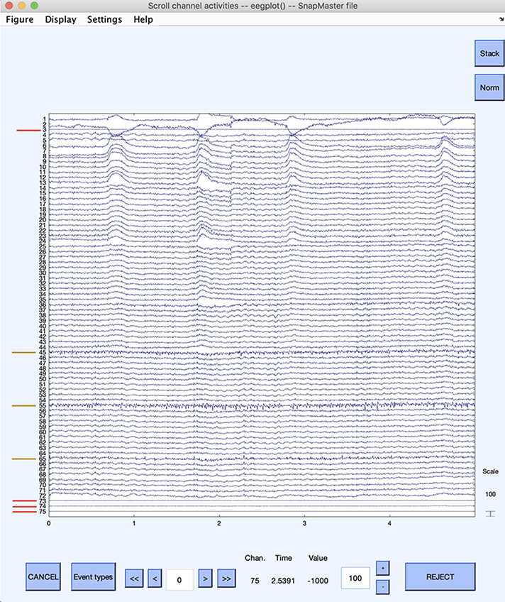
Potentially bad channels are indicated above with red lines for channels 3, 73, 74, 75 (flat channels), and 45, 55, 65 (noisy channels). Channels 45 and 55 seem to have higher noise content than channel 65. The colored lines were added with Photoshop and are not be visible on the channel scrolling interface. When visually identifying bad channels, you should scroll through the whole dataset, as some channels may only be bad for short periods. In this case, it might be preferable to remove the corrupted data segment than the channel itself. Removing a channel that is only transiently bad is also a trade-off with the number of channels available. When a large number of channels are available, one may easily remove a few channels.

Once you have identified bad channel indices or labels, you may use instructions to remove these channels in the final section of this page.

Looking data spectrum

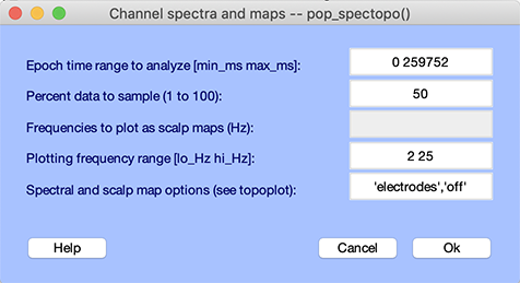
Another way to identify bad channels is to plot the channels’ spectra. To plot the channel spectra, select Plot → Channel spectra and maps. The interface below pops up. Simply press Ok.

Image:plot_spectrum_bad_chan.png

The following window pops up.

Image:plot_spectrum_bad_chan2.png

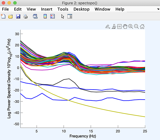
In this window, it is possible to click on individual channel traces, and the channel index is shown on the MATLAB command line. In this case, we see that the bottom four channels are outliers. Clicking on the channel traces reveals that these are channels 3, 73, 74, and 75. There are also two channels with high-frequency noise (the purple and blue trace). These are channels 45 and 55. This confirms bad channels visually identified in the previous section – although in this case, channel 65 does not appear to be an outlier.

Reject channels by index or label

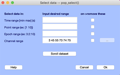
If you know which channels are bad, you may reject them using the function pop_select.m called by selecting the Edit → Select data mneu item. In the example below, we remove channel 3, 45, 55, 73, 74, and 75 identified in the previous sections.

Image:pop_select_new.png

Press Ok to remove the channels. Now a pop_newset.m window for saving the new dataset pops up. We name this new dataset “Dataset cleaned of bad channels” and press Ok.

Channel labels and channel indices

EEGLAB uses both channel labels and channel indices. The EEG dataset we processed in this section did not have channel labels. However, the tutorial dataset has channel labels. You may use the File → Load existing dataset menu item to import tutorial file “eeglab_data.set” in the “sample_data” folder.

To find the correspondence, use the channel editor Edit → Channel locations. You may also plot the electrode names and locations by selecting Plot → Channel locations → By name, producing the figure below.

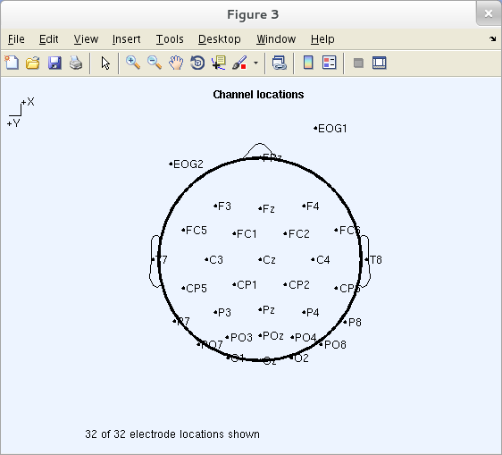
Click on a channel label (for example, POz) to display its number (27).