In previous analyses, the repetition levels were either averaged or used as a categorical variable. Here, we instead used the time between each repetition of the same stimulus – thus for a given subject we have 3 conditions (familiar faces, unfamiliar faces and scrambled faces) and one continuous variable (the distance between the repeat of a stimulus type).

1st level

For this design, we consider 3 conditions: familiar faces, scrambled faces, and unfamiliar faces; along with one continuous variable: the distance between repetitions (in trials). From STUDY, create a new design and let’s call it ‘Repetition’ and then click ‘new’ to add conditions (figure 42).

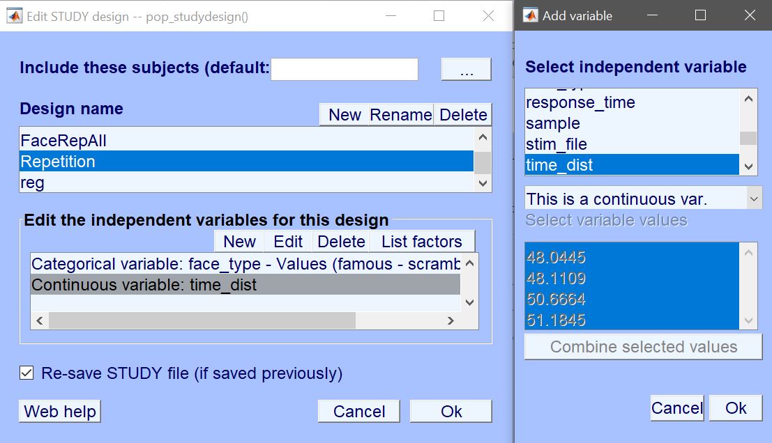Figure 42. Building a STUDY with a continuous variable.

Given that we are interested in repetition, why adding the face type? By modelling repetition as a single variable, we expect trials to covary the same whatever the type of stimulus. Since we know faces activates more than scrambled faces, the slope of the regression will be affected by this difference – and so this is important to also include the conditions. One can also split the time regressor with face type, which will split the time regressor into three continuous regressors and we can recombine them using a contrast. This is available when estimating limo parameters (figure 43 for ERP, Spectrum, and ERSP).

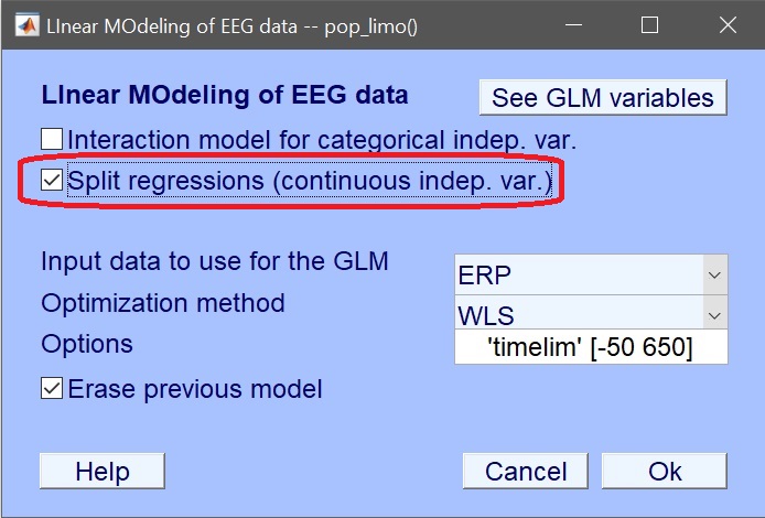
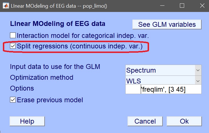
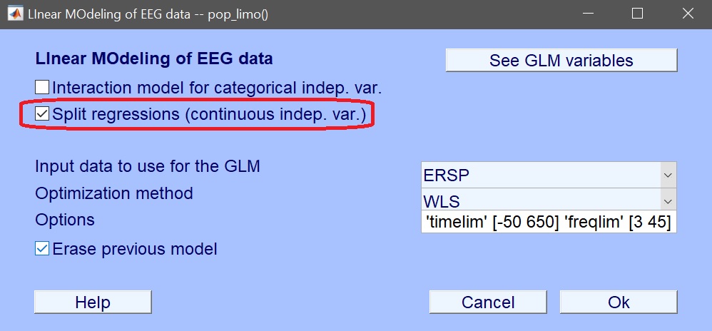
Figure 43. Estimate parameters - splitting continuous variable by the categorical one.

After estimating the models, you can check the design matrix using limo –> results –> review design (figure 44), showing the time between trials split for each condition.

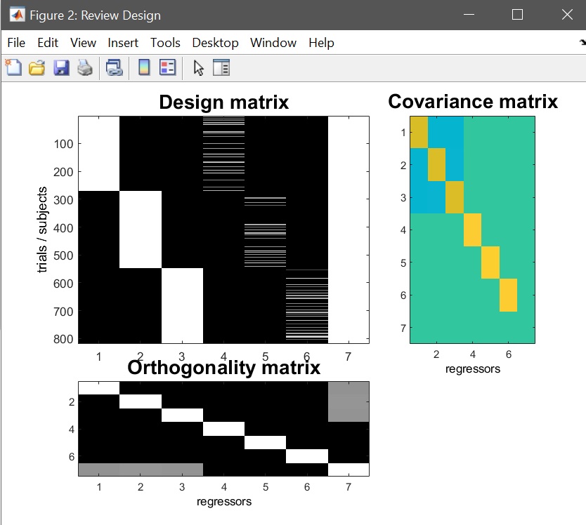
Figure 44. Design matrix for one subject.

You can create and estimate this design with these command lines

STUDY = std_makedesign(STUDY, ALLEEG, 2, 'name','Face_time','delfiles','off','defaultdesign','off',...
    'variable1','face_type','values1',{'famous','scrambled','unfamiliar'},'vartype1','categorical',...
    'variable2','time_dist','values2',[],'vartype2','continuous',...
    'subjselect',{'sub-002','sub-003','sub-004','sub-005','sub-006','sub-007','sub-008','sub-009','sub-010','sub-011','sub-012','sub-013','sub-014','sub-015','sub-016','sub-017','sub-018','sub-019'});
[STUDY, EEG] = pop_savestudy( STUDY, EEG, 'savemode','resave');
STUDY = pop_limo(STUDY, ALLEEG, 'method','WLS','measure','daterp','timelim',[-50 650],'erase','on','splitreg','on','interaction','off');

2nd level

To test the effect of time (i.e. repetition), we are using a one-way repeated measure ANOVA. This will test if there is a difference based on the stimulus type in the way repetition influence linearly EEG activity. For that from the 2nd level GUI (figure 9), select a new directory, load channel location file, click on ANOVA, choose repeated measures, full scalp, enter model parameters: 1 for group and 3 to indicate one factor of three levels and select the beta parameters list for the repetition design – using parameters 4 5 6 see one-way ANOVA tutorial for details. Next, go the limo results and create a new contrast, we test here if this effect differs for familiar faces using a contrast [2 -1 -1] (figure 45).

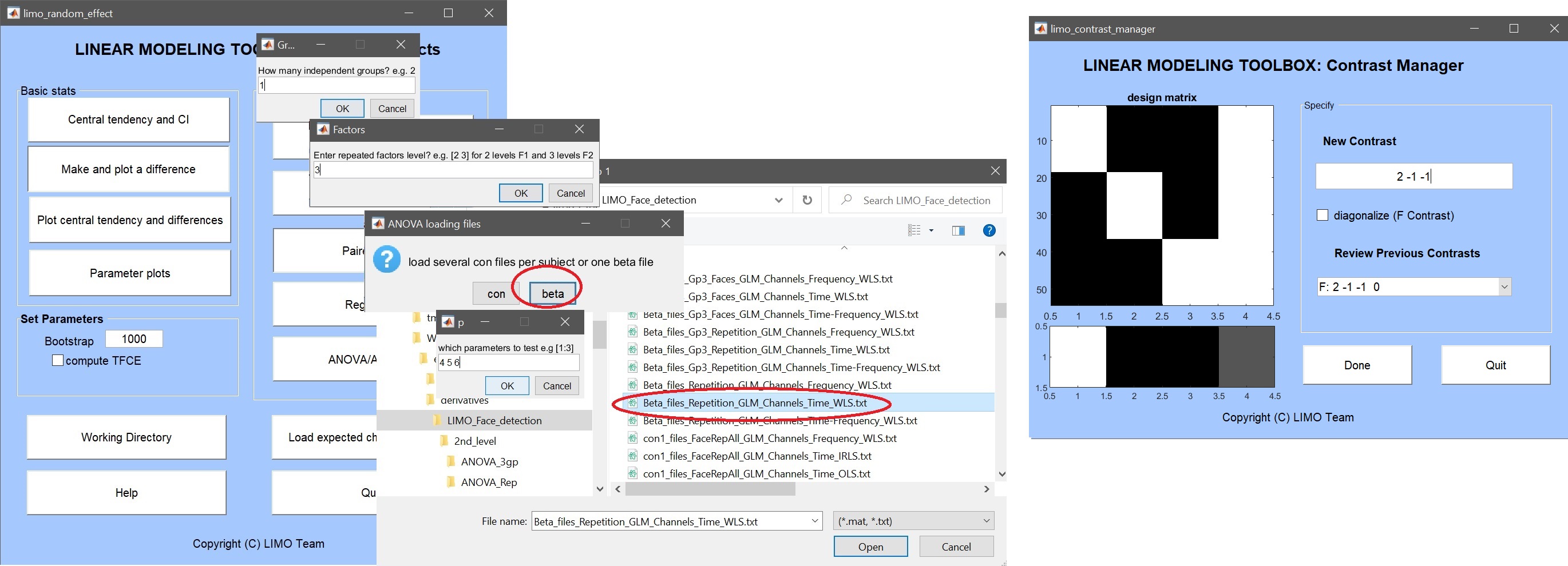
Figure 45. One-way ANOVA on repetition regression parameters.

Results of the ANOVA show when/where repetition effects differ between condition (the regression of the trial distance on trials for famous faces vs scrambled faces vs unfamiliar faces), and results from the contrast that this is driven by a repetition effect for famous faces.

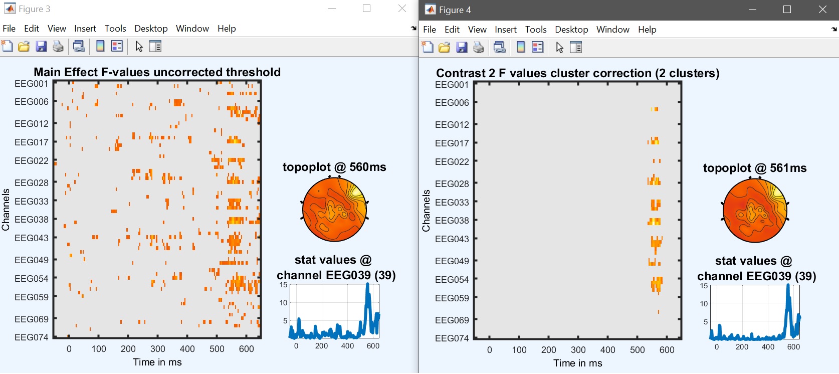
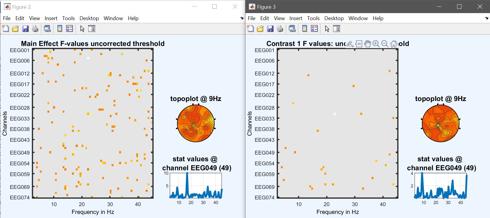
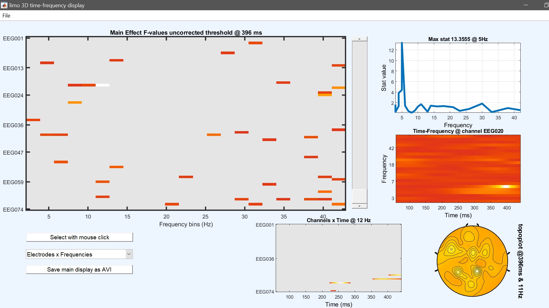
Figure 46. One-way ANOVA and contrasts results for repetition regression parameters.