Plotting Event Related Potentials
EEGLAB contains several functions for plotting 1-D ERP averages of dataset trials (i.e., epochs). EEGLAB also features functions for studying the EEG dynamics expressed in the single trials. This may be visualized, in large part, via 2-D (potential time series by trials) ERP image transforms of a dataset of single-trial epochs (a.k.a., epoched data) as detailed in the following section of the tutorial.
Table of contents
Plotting the ERP data on a single axis with scalp maps
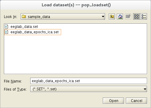
We use here the tutorial dataset as it was after extracting data epochs. Select menu item File and press sub-menu item Load existing dataset. Select the tutorial file “eeglab_data_epochs_ica.set” located in the “sample_data” folder of EEGLAB. Then press Open.
Plotting all-channel ERPs
To plot the average ERP of all dataset epochs, plus ERP scalp maps at selected latencies, select Plot → Channel ERPs → With scalp maps. As a simple illustration using the sample dataset, we retain the default settings in the resulting pop_timtopo.m window below, and press Ok.

A figure (below) appears. Each trace plots the averaged ERP at one channel. The scalp map shows the topographic distribution of the average potential at 430 ms (the latency of maximum ERP data variance). Alternatively, one or more exact scalp map latencies may be specified in the pop-window above.
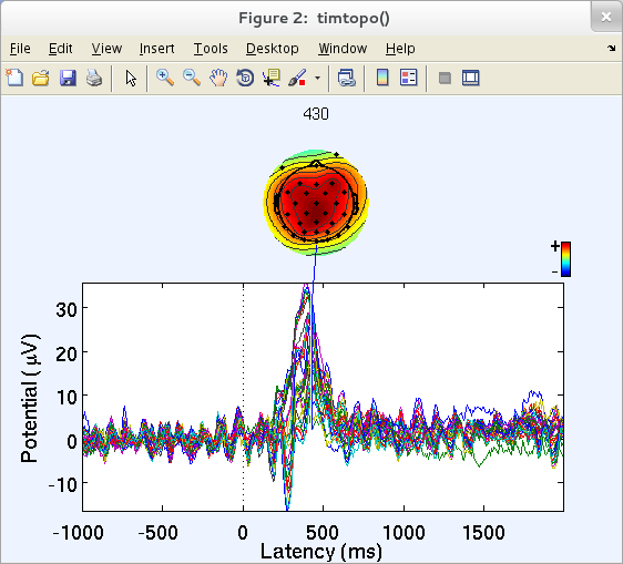
The pop_timtopo.m function plots the relative time courses of the averaged ERP at all channels, plus ‘snapshots’ of the scalp potential distribution at various moments during the average ERP time course. Clicking on one of the traces above will plot the scalp topography at the corresponding latency. Note that to visualize the ERP scalp map at all latencies as an ERP movie (i.e., to view the play of the ERP on the scalp), use function eegmovie.m from the command line as described in the scripting section of the tutorial.
Plotting ERPs in a Topographic Map
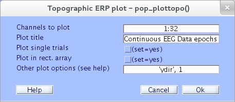
Here we will plot the ERPs of an epoched dataset as single-channel traces in their 2-D topographic arrangement. Select Plot → Channel ERPs → In scalp array/rect. array. Using the default settings and pressing Ok in the window below.
This produces the following pop_timtopo.m figure.
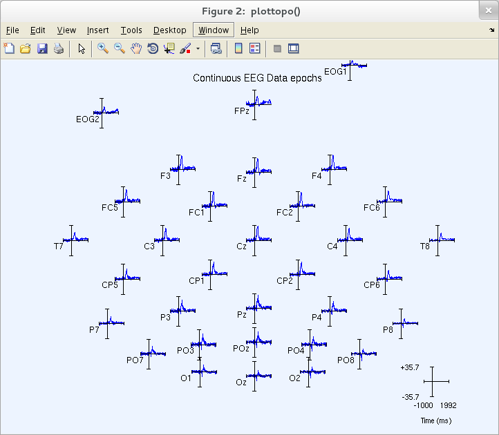
You may visualize a specific channel time course by clicking on its trace (above), producing a pop-up sub-axis view. For example, click on the ERP trace marked POz (above) to call up a full-sized view of this trace (as below).
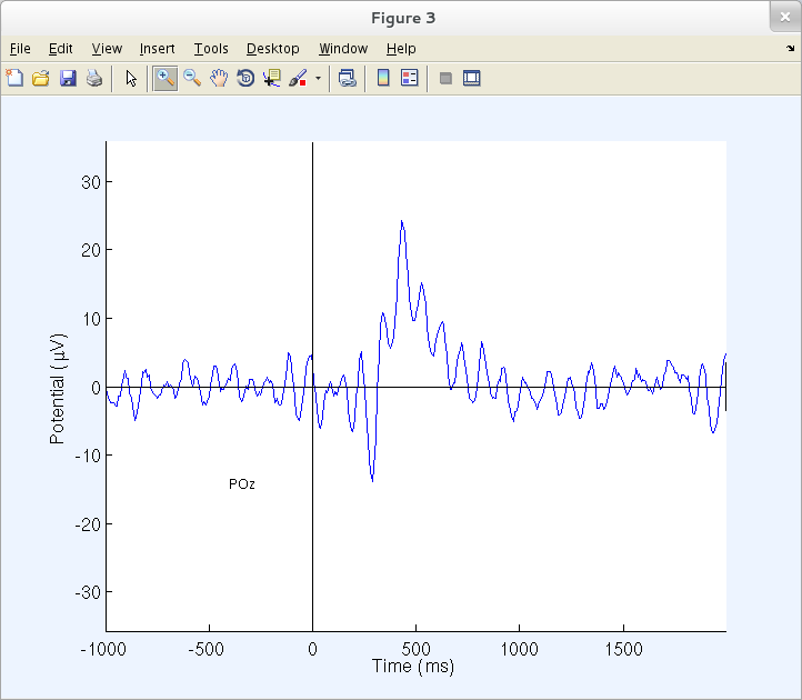
Many EEGLAB plotting routines use the toolbox function axcopy.m to pop up a sub-axis plotting window whenever users click on the main plot window. Sub-axis windows do not have axcopy.m enabled, allowing the user to use the standard MATLAB mouse ‘Zoom In/Out’ feature.
Plotting ERPs in a Column Array
To plot (one or more) average ERP data traces in two-column arrays, select menu item Plot → Channel ERPs → In scalp/rect. array. To use the default settings in the resulting window, check the “Plot in rect. array” checkbox and press Ok.

The resulting pop_plottopo.m figure (below) appears.
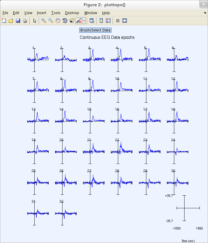
As in the previous plot, clicking on a trace above pops up a full window sub-axis view.
Plotting a series of 2-D ERP scalp maps
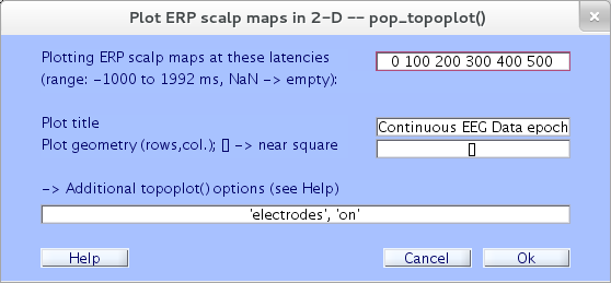
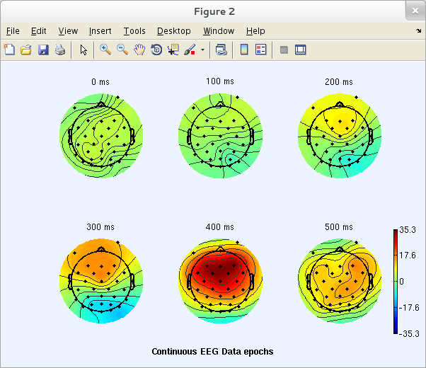
Here we will plot ERP data for a series of 2-D scalp maps representing potential distributions at a selected series of trial latencies. Select Plot → ERP map series → In 2-D. In the top text box of the resulting pop_topoplot.m window (below), type the epoch latencies of the desired ERP scalp maps.
Note that in this or any other numeric text entry box, you may enter any numeric MATLAB expression. For example, instead of 0 100 200 300 400 500, try 0:100:500. Even more complicated expressions, for example -6000+3*(0:20:120), are interpreted correctly.
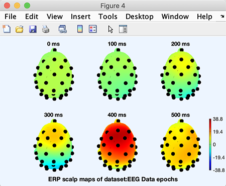
The window (below) then appears, containing ERP scalp maps at the specified latencies. Here, the plot grid has 3 columns and 2 rows; other plot geometries can be specified in the GUI window above via the Plot geometry text box.
Plotting a series of 3-D ERP scalp maps
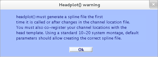
To plot ERP data as a series of 3-D scalp maps, go to the menu Plot → ERP map series → In 3-D. The query window (below) will pop up, asking you to create and save a new 3-D head map 3-D spline file. This process must be done only once for every montage. Click Ok to begin this process.
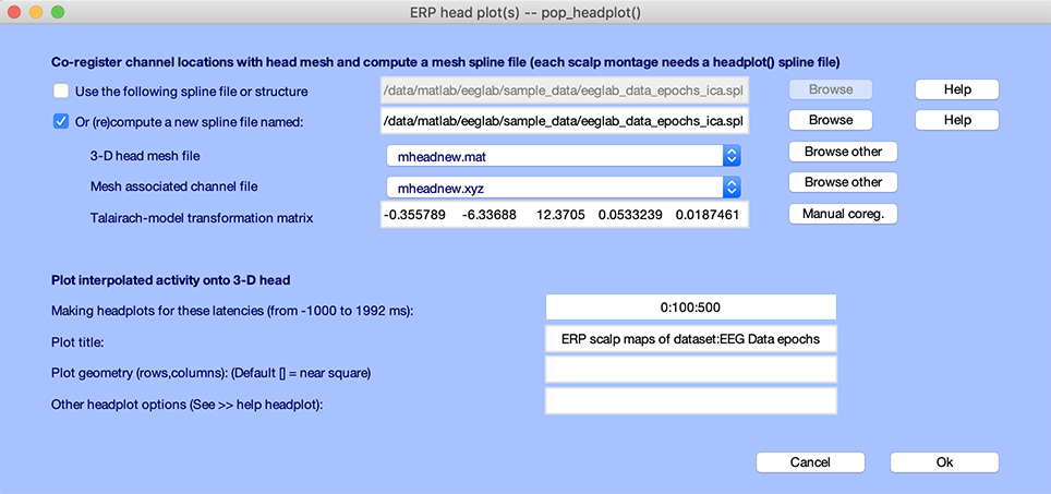
The window below will pop up. Because we use template electrode locations, the conversion between channel location and 3-D headplot coordinate (Talairach-model transformation matrix entry) is automatically filled in. If this is not the case, refer to the following section on aligning the 3-D head plot to your electrode coordinate system.
Enter trial latencies to be plotted (0:100:500 below indicating latencies 0, 100, 200, 300, 400, and 500 ms) and press Ok.
Now, the 3-D plotting function pop_headplot.m, will create the 3-D channel locations spline file. A progress bar will pop up to indicate when this process will be finished. When the 3-D spline file has been generated, the following plot will appear.
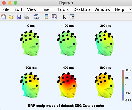
As usual, clicking on a head plot will make it pop up in a sub-axis window in which it can be rotated using the mouse. Note that to select (for other purposes) a head plot or other object in a figure with the axcopy.m pop-up feature activated, click on it, then delete the resulting pop-up window.
To plot the heads at a specified angle, select again the Plot → ERP map series → In 3-D menu item. By default, the function uses the 3-D spline file you have generated above. Enter latencies to be displayed and the headplot.m ‘view’ option (as in the example below), and press Ok.
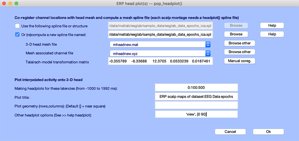
The headplot.m window (below) will then appear. You may also rotate the individual heads using the mouse. This is often necessary to best show the illustrated spatial distribution.
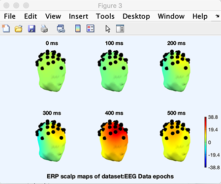
You may also use a different head template. For example, use again the Plot → ERP map series → In 3-D menu item, and select the second template model Colin27headmesh.mat in the 3-D mesh file list box (you may also browse for your own 3-D mesh file using the Browse other button). Again select latencies to be plotted (0:100:500) and press Ok. Now the result is being plotted on a different head model.
Co-registration of channel locations with head model
Select again the Plot → ERP map series → In 3-D menu item. If you have already generated a spline file for this channel location structure, you may enter it here in the first edit box (first click on the Use existing spline file or structure to activate the edit box, then browse for a data file). If you do not have such a file, you will need to generate one.
However, first, your channel locations must be co-registered with the 3-D head template to be plotted. Note that if you are using one of the template channel location files and one of the template head mesh, the Talairach-model transformation matrix field (containing channel alignment information) will be filled automatically, as this was the case in the previous section.
We will now briefly describe the channels-to-head model co-registration process. If your dataset contains channel locations, for example, locations that you may have measured on the subject head using a Polhemus system, and you want to use these electrode locations for 3-D plotting, headplot.m must first determine the positions of your electrode locations relative to a template head surface. A generic transformation cannot be performed because the origin ([0 0 0]) in your electrode location system does not necessarily correspond to the center of the template head (.e.g., the intersection of the fiducial points: nasion and pre-auricular points) used by headplot.m. Even if this were the case, heads have different shapes, so your scanned electrode locations might need to be scaled or warped in 3-D to match the template head mesh.
The co-registration window begins this operation. Set the checkbox labeled Or recompute a new spline file named:, and then click the Manual coreg. push button. A window appears explaining how to perform the co-registration.

Pressing Ok will cause the co-registration window below to open.
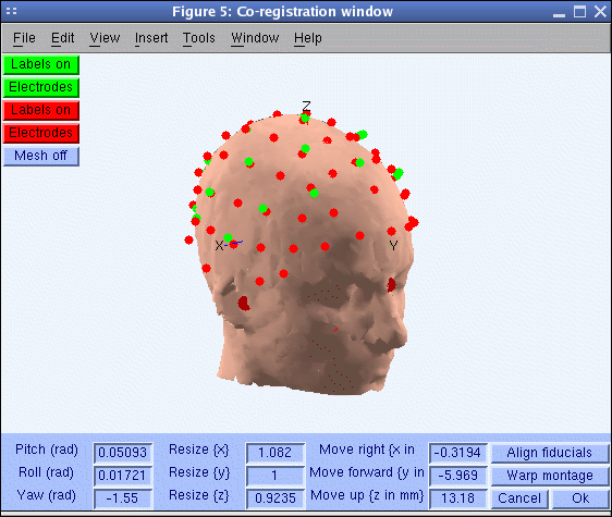
In the window above, the red electrodes are those natively associated with the template head mesh. Rather than directly aligning your electrode locations (shown in green) to the head mesh, your montage will be aligned to template electrode locations associated with the head mesh by scanning on the same subject’s head (here shown in red). For the sample dataset, this alignment has already been performed. (Click the Labels on push button to display the electrode labels).
When you have finished the co-registration, simply click Ok and a vector of 9 new channel alignment values (shift, in 3-D; rotation, in 3-D; scaling, in 3-D) will be copied back to the Talairach-model transformation matrix field of the interactive headplot.m window. For more information about channel co-registration, see the source reconstruction tutorial.
Note that it is possible, and relatively easy, to generate custom headplot.m head meshes. This may be done using Freesurfer or FieldTrip.
Comparing different conditions and performing statistics
Comparing ERPs between conditions is done using group-level analysis even if you only have one subject. This is because the group-level analysis interface has rich options to select and plot ERPs for different conditions, including calculating statistics across trials for single subjects.