Here we will use the three basic conditions to run a group level ANOVA. LIMO runs a hierarchical model, first a GLM at the subject level (first level), second a GLM at the group level (second level). Under some assumptions about the data, this is equivalent to running mixed model analysis on all trials for all subjects with subjects as random effects – but much faster to calculate.

First level analysis

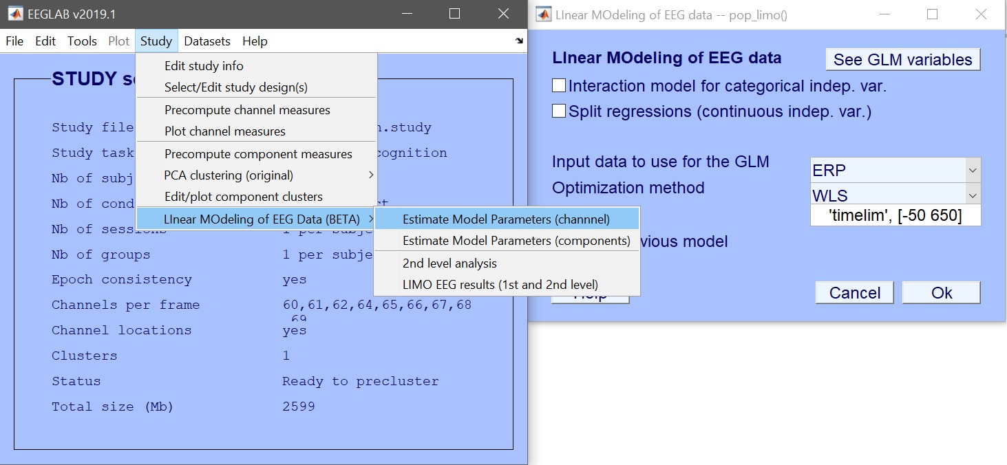
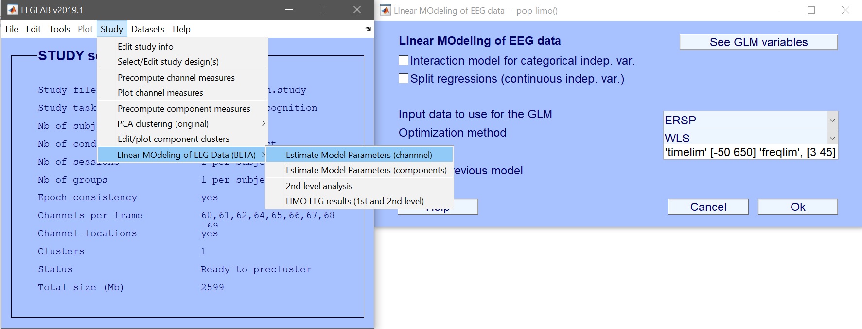
We first create the design – Rename design 1 as ANOVA_Faces and then Delete current variables (figure 6). Click ‘New’ to add variables of interest – here select face type (figure 7). Press OK to add those variables, and OK again to close the design selection. You are ready to create the design in LIMO MEEG and compute the model parameters (figure 8 for ERP, spectrum or ERSP). Input the data type (ERP, Spectrum or ERSP) and possibly restrict the time or frequency range. The default method (Weighted Least Squares) is the preferred options, as long as you have more trials than data frames.

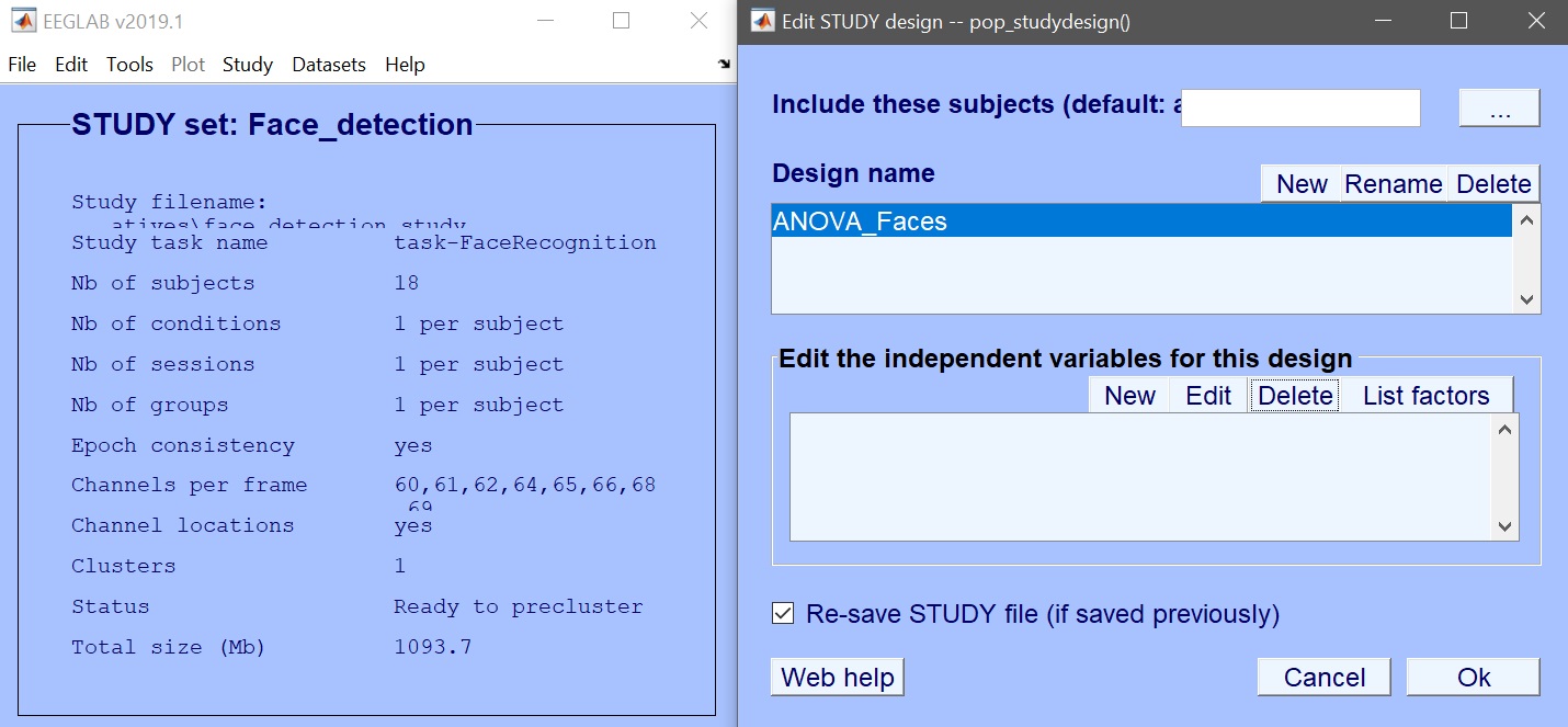Figure 6. Edit design

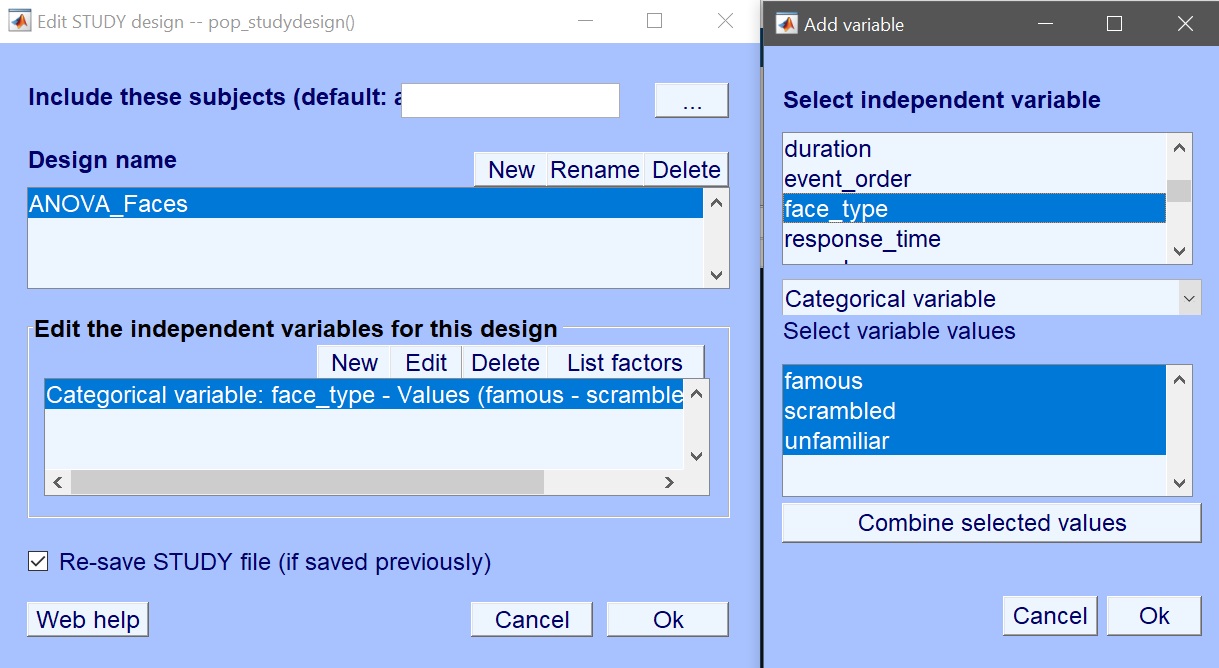Figure 7. Create new design

This can be executed in command line as:

% 1st level analysis - specify the design
% We ignore the repetition levels using the variable 'face_type'
STUDY = std_makedesign(STUDY, ALLEEG, 1, 'name','ANOVA_Faces','delfiles','off','defaultdesign','off',...
    'variable1','face_type','values1',{'famous','scrambled','unfamiliar'},'vartype1','categorical',...
    'subjselect',{'sub-002','sub-003','sub-004','sub-005','sub-006','sub-007','sub-008','sub-009',...
    'sub-010','sub-011','sub-012','sub-013','sub-014','sub-015','sub-016','sub-017','sub-018','sub-019'});
[STUDY, EEG] = pop_savestudy( STUDY, EEG, 'savemode','resave');

Figure 8a. LIMO Estimate model parameters for ERP using Weighted Least Squares (WLS)

STUDY  = pop_limo(STUDY, ALLEEG, 'method','WLS','measure','daterp','timelim',[-50 650],...
    'erase','on','splitreg','off','interaction','off');

Figure 8b. LIMO Estimate model parameters for Spectrum using Weighted Least Squares (WLS)

STUDY  = pop_limo(STUDY, ALLEEG, 'method','WLS','measure','datspec','freqlim',[3 45],...
    'erase','on','splitreg','off','interaction','off');

Figure 8c. LIMO Estimate model parameters for ERSP using Weighted Least Squares (WLS)

STUDY  = pop_limo(STUDY, ALLEEG, 'method','WLS','measure','dattimef',...
    'timelim',[-50 650],'freqlim',[3 45],'erase','on','splitreg','off','interaction','off');

Figure 8. Estimate model parameters

After a few minutes, all subjects are processed: design is build and parameter estimated. All analyses appear within each subject derivatives folder – inside a folder with the name of the design, the measure analysed, space, and the method used, for instance /derivatives/sub-002/eeg/ ANOVA_Faces_GLM_Channels_Time_WLS

Inside are the extracted data (Yr.mat), the modelled data (Yhat.mat), model parameters (Betas.mat), model residuals (Res.mat), model fit (R2.mat), statistical effect (condition_effect_1.mat) and model information itself (LIMO.mat).

There are also a few other useful files:

LIMO_face_detection is a folder with the txt files listing all the files used and generated, these are useful for group level analyses
LIMO_face_detection/limo_batch_report is a folder that contains the psom batch files and list which files failed in any – also contains the psom pipeline.

The above analyses can be executed in command line as:

2nd level analysis

For each subject, there are 4 model parameters (Betas): familiar, scrambled, unfamiliar (stored in the order it appears when you make the design) and the last parameter is the subject-specific constant. Doing a 1-way ANOVA consists simply in entering these beta values (files) and setting this as a single factor with 3 levels.

Click on Study –> Linear MOdeling of EEG Data –> 2nd level analysis (figure 9).

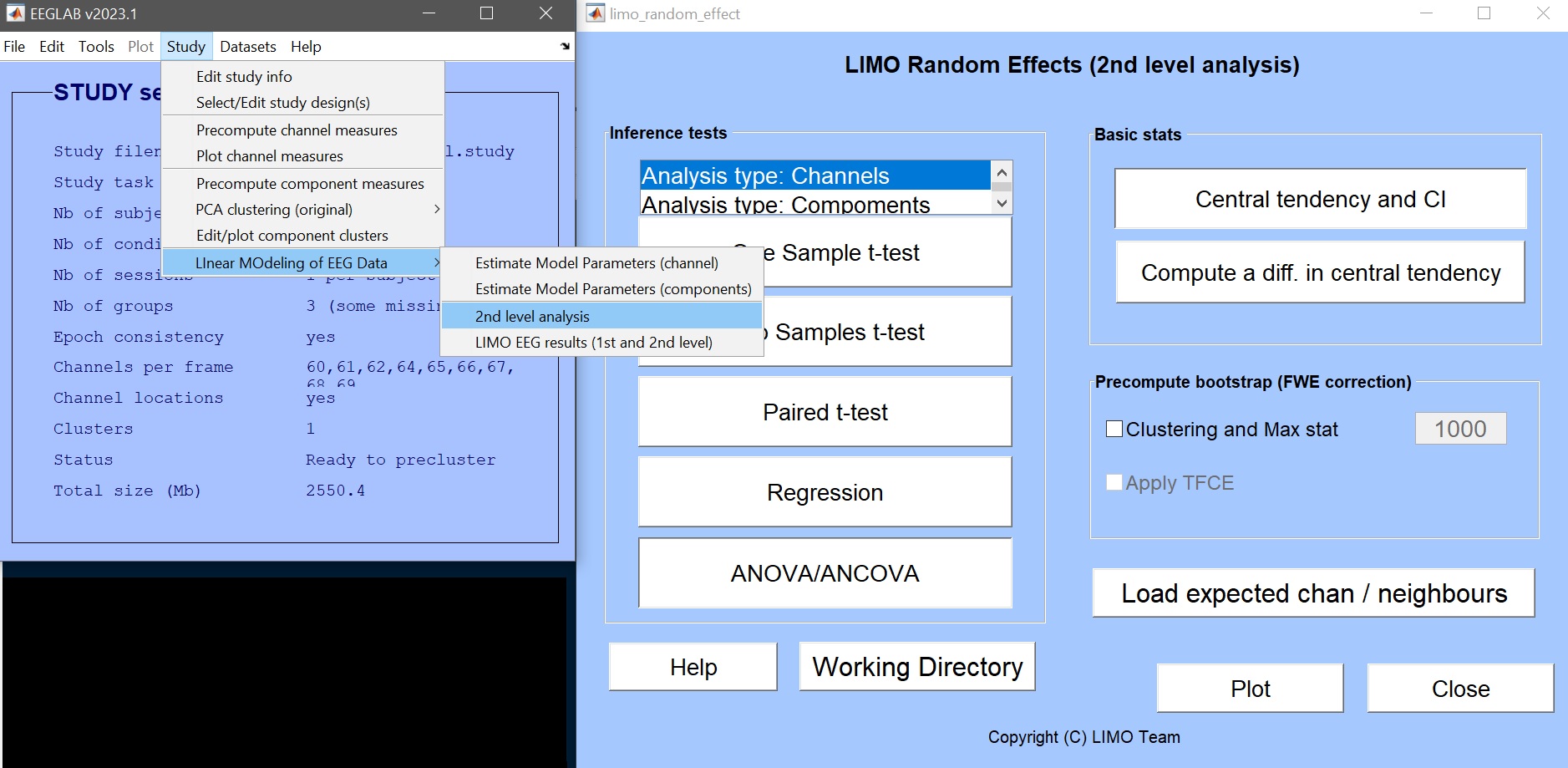Figure 9. Calling LIMO 2nd level

load the group level channel location file – this should be located at the root of the derivatives folder (figure 10)
make a new directory (‘1way_ANOVA’) to save this new analysis and select this as a working directory (figure 11)
click on ANOVA/ANCOVA (figure 12) and fill the information as needed: Full scalp analysis –> Repeated measure ANOVA –> 1 group –> 1 factor of 3 levels
select beta files, enter which beta to analyse [1 2 3], and name that factor ‘faces’ (figure 13)

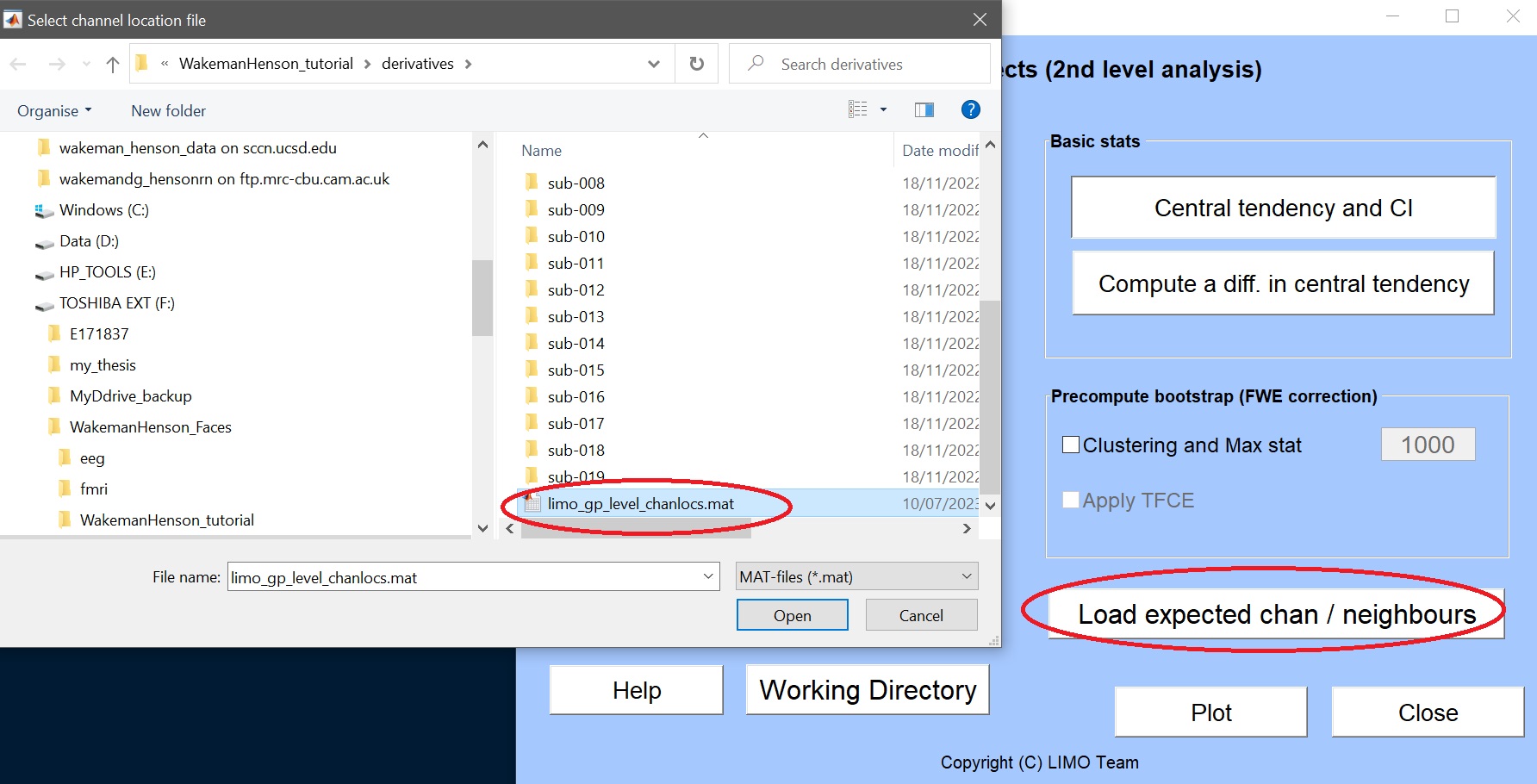Figure 10. load group level channel location file

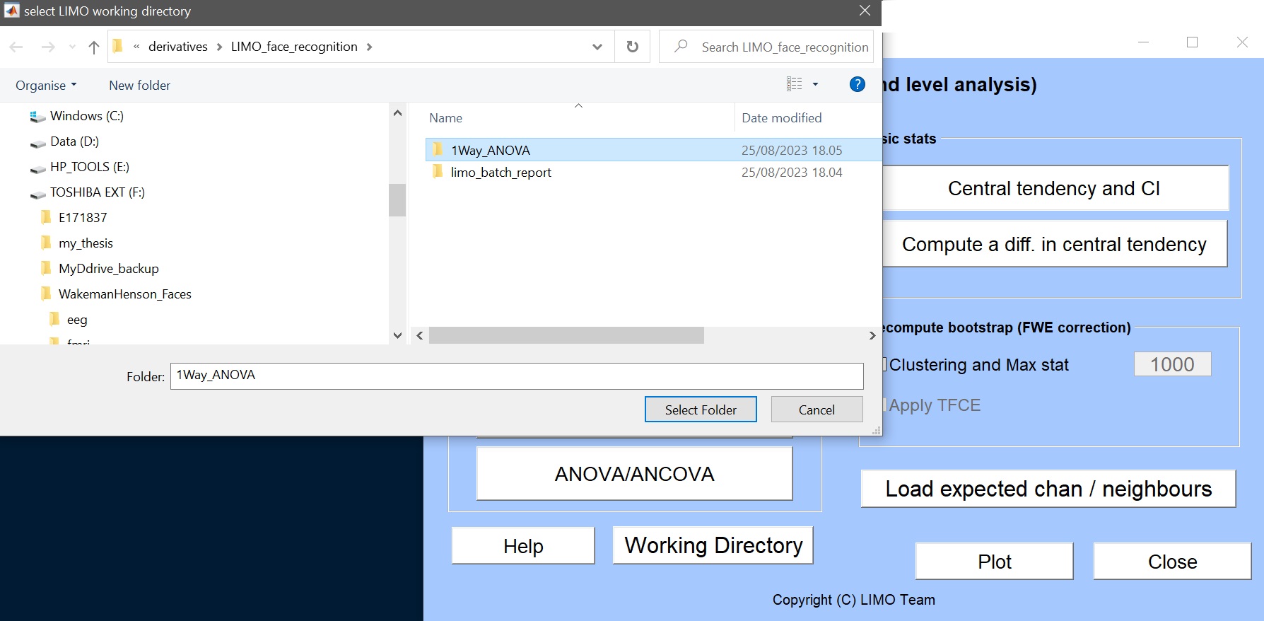Figure 11. Select working directory

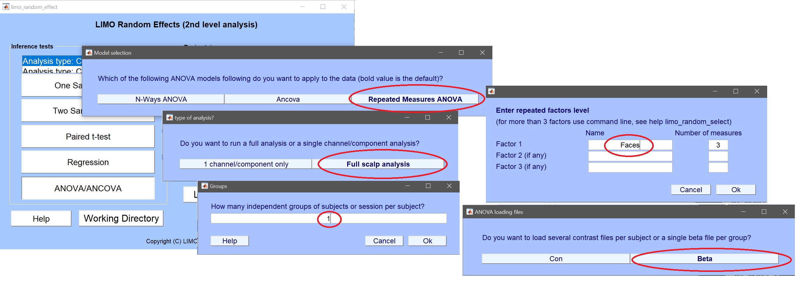Figure 12. Setting up a 1 Way repeated measure ANOVA

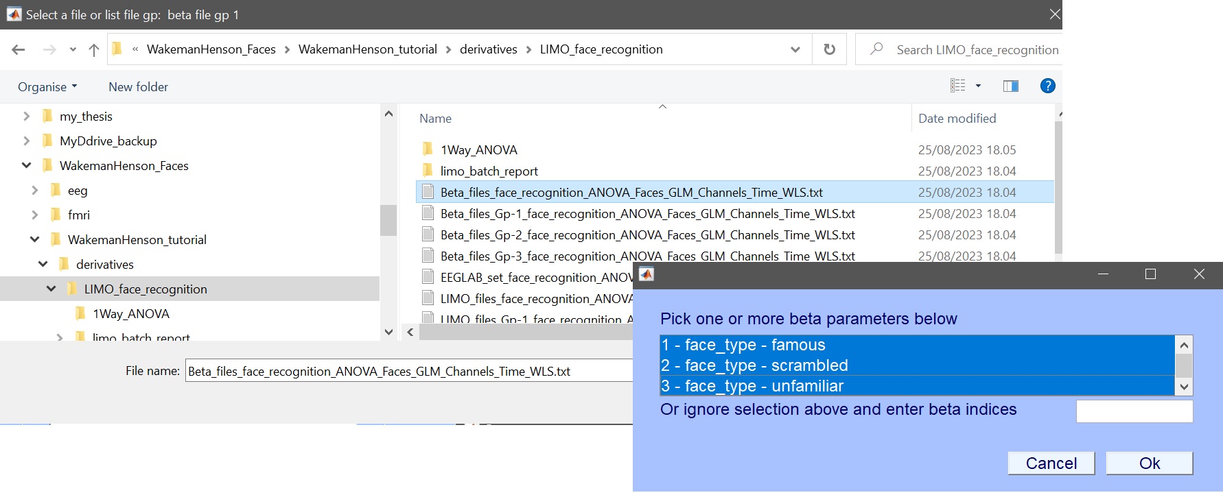Figure 13. Select beta files (here shown for ERP, i.e. Channels Time WLS) and parameters

The design matrix should then pop up (figure 14), and answer ‘yes’ to start the analysis.

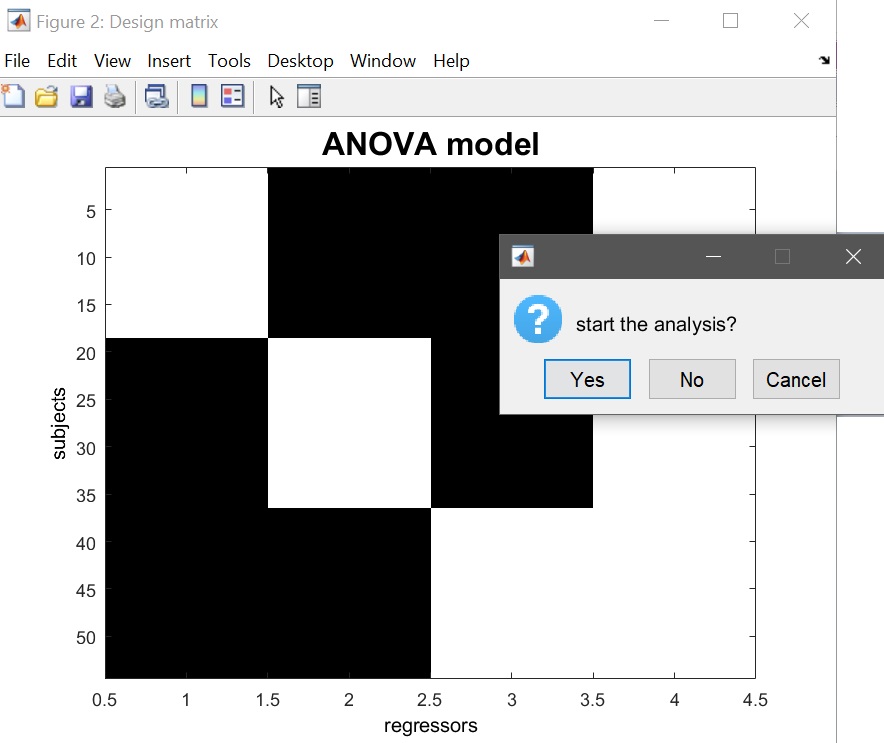Figure 14. 1-way ANOVA Design matrix (1 column per condition + constant term)

These steps can be executed in command line as:

% 2nd level analysis - ANOVA on Beta parameters 1 2 3
chanlocs = [STUDY.filepath filesep 'limo_gp_level_chanlocs.mat'];
mkdir([STUDY.filepath filesep '1-way-ANOVA'])
cd([STUDY.filepath filesep '1-way-ANOVA'])
% ERP
limo_random_select('Repeated Measures ANOVA',chanlocs,'LIMOfiles',...
    {[STUDY.filepath filesep 'LIMO_Face_detection' filesep 'Beta_files_ANOVA_Faces_GLM_Channels_Time_WLS.txt']},...
    'analysis_type','Full scalp analysis','parameters',{[1 2 3]},...
    'factor names',{'face'},'type','Channels','nboot',1000,'tfce',0,'skip design check','yes');
% Spectrum
limo_random_select('Repeated Measures ANOVA',chanlocs,'LIMOfiles',...
    {[STUDY.filepath filesep 'LIMO_Face_detection' filesep 'Beta_files_ANOVA_Faces_GLM_Channels_Frequency_WLS.txt']},...
    'analysis_type','Full scalp analysis','parameters',{[1 2 3]},...
    'factor names',{'face'},'type','Channels','nboot',1000,'tfce',0,'skip design check','yes');
% ERSP
limo_random_select('Repeated Measures ANOVA',chanlocs,'LIMOfiles',...
    {[STUDY.filepath filesep 'LIMO_Face_detection' filesep 'Beta_files_ANOVA_Faces_GLM_Channels_Time-Frequency_WLS.txt']},...
    'analysis_type','Full scalp analysis','parameters',{[1 2 3]},...
    'factor names',{'face'},'type','Channels','nboot',1000,'tfce',0,'skip design check','yes');

Exit the 2nd level GUI and call LIMO results by pressing the “Plot” button) which will ask what to plot and will automatically propose the ANOVA result.

Plot button -- calls to plot results

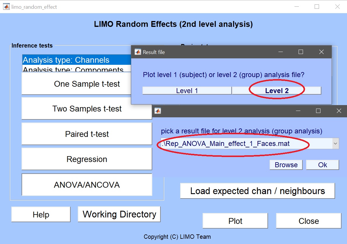
By default, the bootstrap option is ‘off’ and thus the ANOVA should compute very quickly. In the 1-way ANOVA folders, several files have been created: the data (Yr.mat), the statistical effects (Rep_ANOVA_Main_effect_1_faces.mat) and model information itself (LIMO.mat).

Choose the multiple comparison method (e.g. clustering) and this will then compute the bootstrap (does that only once). After a while the figure is updated. A new H0 folder is there, with the resampling table (boot_table.mat), the null data (centered_data.mat), and the bootstrapped statistical results under H0. Results for the different clusters are also reported in the command window.

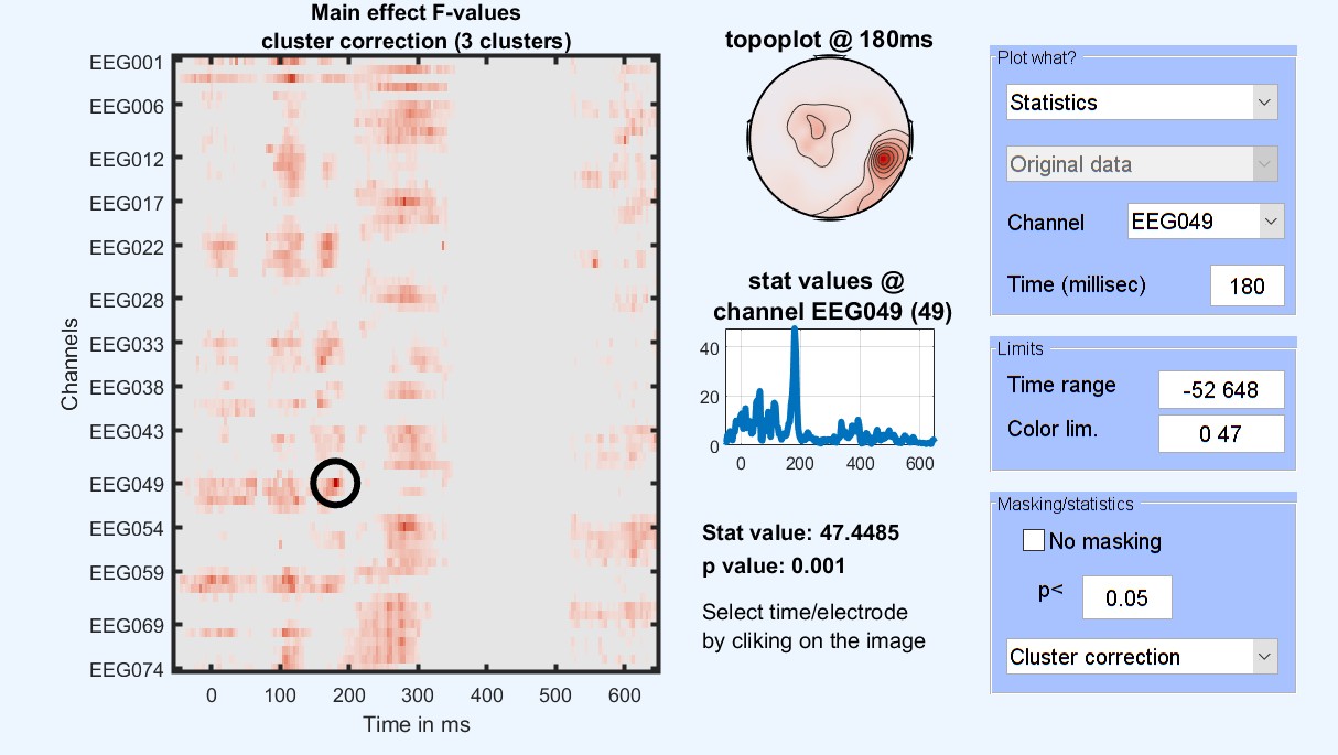
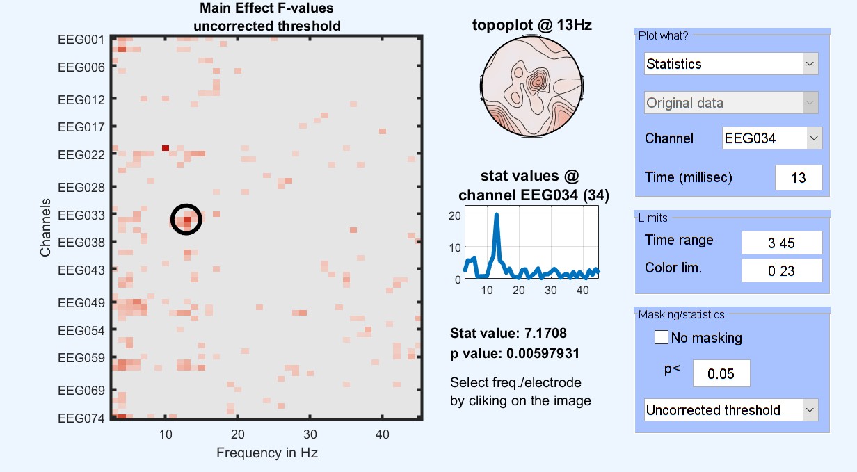
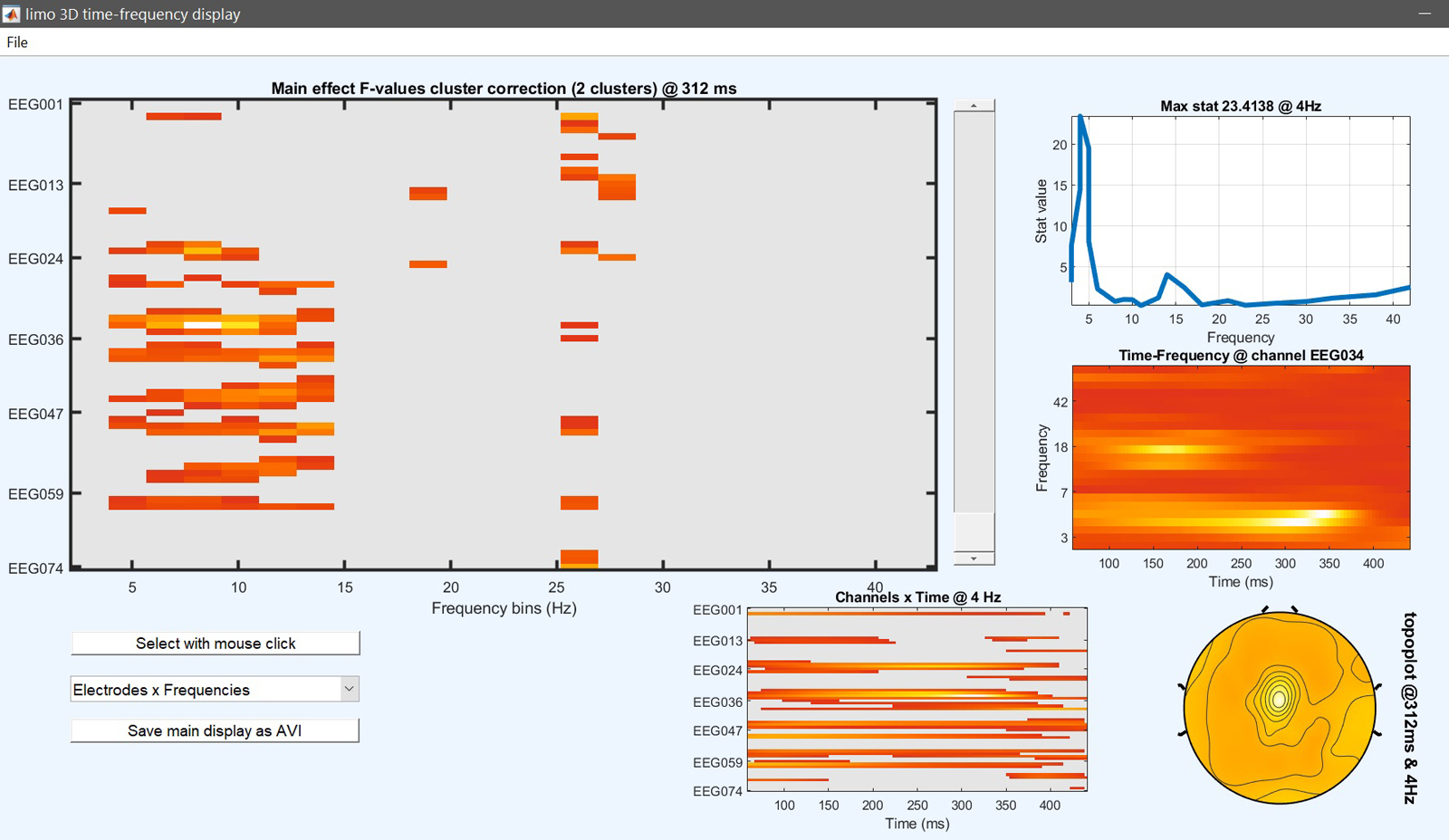Figure 15. 1-way ANOVA ERP Results for famous faces vs scrambled vs unfamiliar Figure 15. 1-way ANOVA Spectrum Results for famous faces vs scrambled vs unfamiliar Figure 15. 1-way ANOVA ERSP Results for famous faces vs scrambled vs unfamiliar Figure 15. 1-way ANOVA Results for famous faces vs scrambled vs unfamiliar

Contrasts

At this stage, the ANOVA results tell us where and when those three conditions differ. To check which condition differs from the other, post-hoc contrasts can be performed testing between pairs of conditions: familiar faces vs. scrambled faces [1 -1 0], unfamiliar faces vs scrambled faces [0 -1 1] and familiar faces vs unfamiliar faces [1 0 -1]. More complex contrasts are also possible, let’s try faces vs scrambled [0.5 -1 0.5] which compare images containing faces with images not containing faces. This is the same type of contrast/post-hoc analysis that you would run in your statistical software.

From the main LIMO MEEG GUI or the result GUI, click on contrast manager and select the “LIMO.mat” file created for the ANOVA. The contrast manager shows the design matrix and we can enter the contrast to compute (figure 16) and click ‘Done’. The contrast and associated bootstrap are then computed. Note that these analyses differ from performing ad-hoc t-tests (see below), mostly because (i) they are computed within the repeated ANOVA model, i.e. accounting for all conditions and (ii) they are not directional relying on a F statistic (ie saved as ess* files).

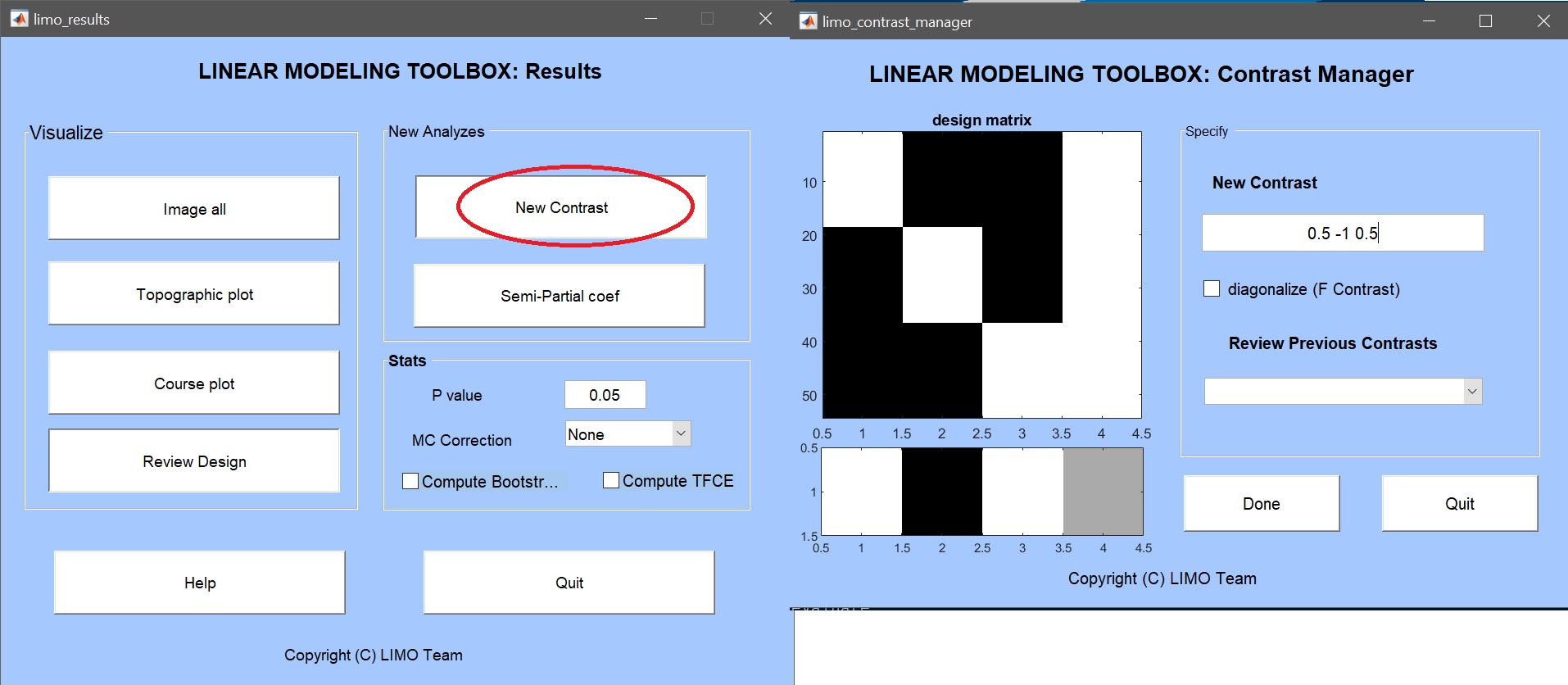Figure 16. Contrast manager showing the design matrix (in white: familiar faces, scrambled faces, unfamiliar faces, constant) and the contrast familiar faces > scrambled faces.

This step can be executed in command line as:

% add contrast famous+unfamiliar>scrambled
limo_contrast(fullfile(pwd,'Yr.mat'),fullfile(pwd,'LIMO.mat'), 3 ,[0.5 -1 0.5]); % compute a new contrast
limo_contrast(fullfile(pwd,'Yr.mat'),fullfile(pwd,'LIMO.mat'), 4);               % do the bootstrap of the last contrast

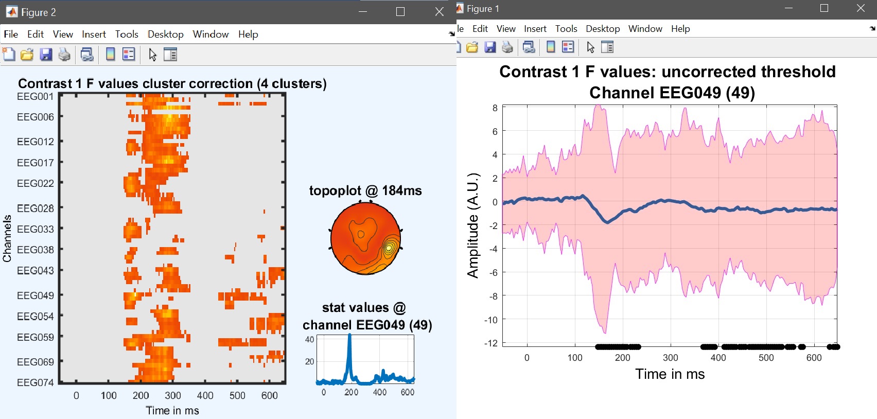
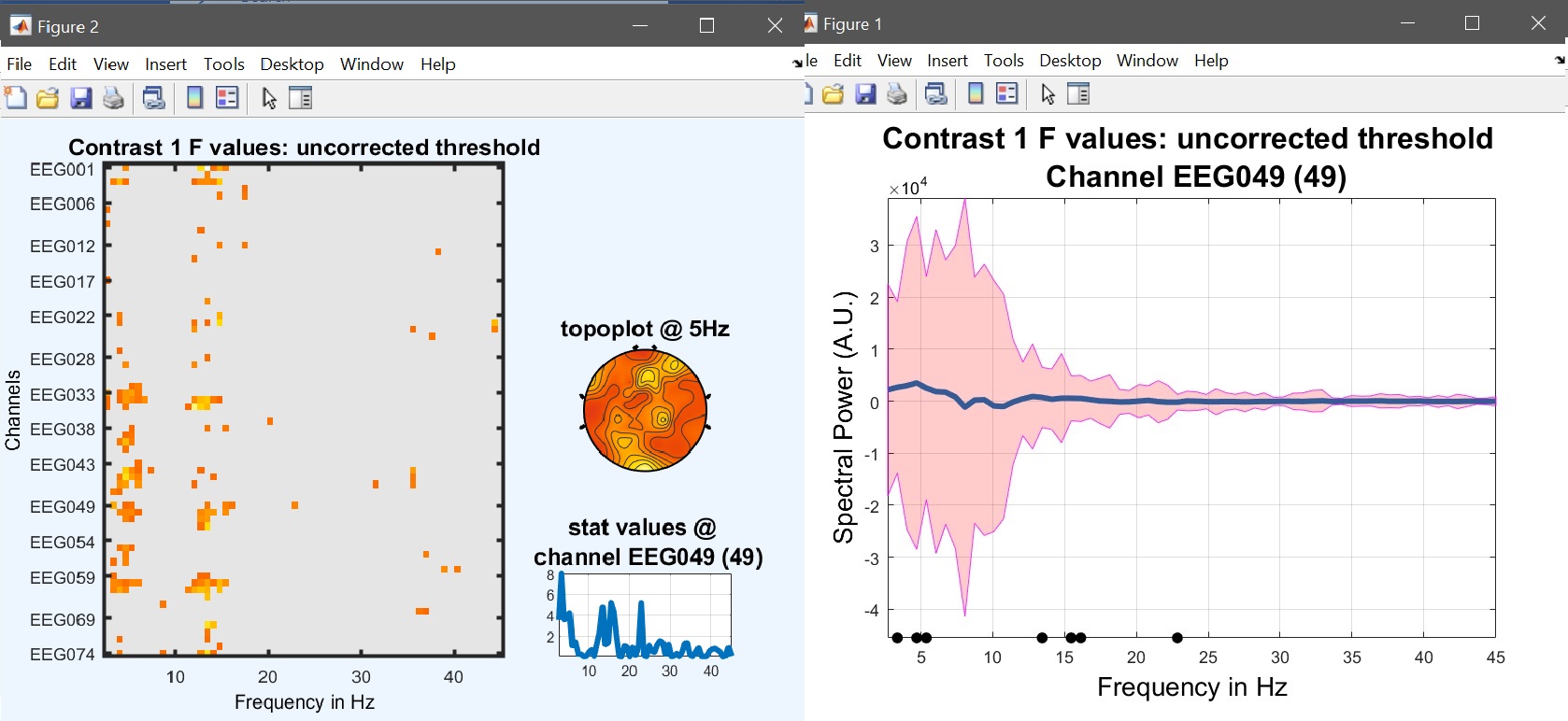
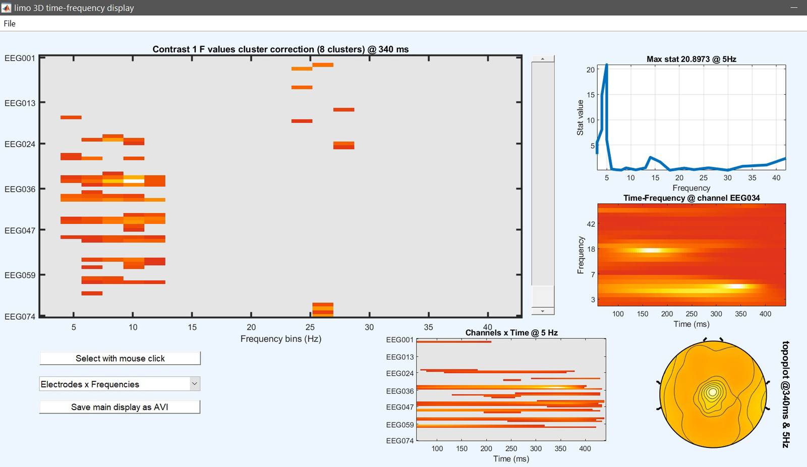
Results can then be viewed again by selecting the newly created ‘ess*.mat’ file using ‘image all’ and using the ‘course plot’ which shows the time course of the difference (figure 17 for ERP, Spectrum and ERSP).

Figure 17a. Contrast ERP results

limo_eeg(5,pwd) % channel*time imagesc for both effects and contrast
limo_display_results(3,'ess_1.mat',pwd,0.05,2,fullfile(pwd,'LIMO.mat'),0,'channels',49); % course plot
saveas(gcf, 'contrast_timecourse.fig'); close(gcf)

Figure 17b. Contrast Specrum results

limo_eeg(5,pwd) % channel*time imagesc for both effects and contrast
limo_display_results(3,'ess_1.mat',pwd,0.05,2,fullfile(pwd,'LIMO.mat'),0,'channels',49); % course plot
saveas(gcf, 'contrast_specprofile.fig'); close(gcf)

Figure 17c. Contrast ERSP results

limo_eeg(5,pwd) % channel*time imagesc for both effects and contrast
limo_display_results(3,'ess_1.mat',pwd,0.05,2,fullfile(pwd,'LIMO.mat'),0,'channels',49); % course plot
saveas(gcf, 'contrast_timecourse.fig'); close(gcf)

Figure 17. Results for the contrast [0.5 -1 0.5 0] i.e. (faces - scrambled)≠0