Advanced plotting from the command line
In this section, you may obtain custom plots from the MATLAB command line. It is currently not possible to obtain these plots from the EEGLAB menus.
Table of contents
Time-frequency plot on all electrodes
This example demonstrates some of the power of low-level scripting that goes beyond the scope of functions currently available through the graphical interface. Below we run this script on the tutorial epoched dataset. The tftopo.m function is a powerful function that allows plotting time-frequency decompositions across all channels.
% Compute a time-frequency decomposition for every electrode
eeglab; close; % add path
eeglabp = fileparts(which('eeglab.m'));
EEG = pop_loadset(fullfile(eeglabp, 'sample_data', 'eeglab_data_epochs_ica.set'));
for elec = 1:EEG.nbchan
    [ersp,itc,powbase,times,freqs,erspboot,itcboot] = pop_newtimef(EEG, …
    1, elec, [EEG.xmin EEG.xmax]*1000, [3 0.5], 'maxfreq', 50, 'padratio', 16, ...
    'plotphase', 'off', 'timesout', 60, 'alpha', .05, 'plotersp','off', 'plotitc','off');
    if elec == 1  % create empty arrays if first electrode
        allersp = zeros([ size(ersp) EEG.nbchan]);
        allitc = zeros([ size(itc) EEG.nbchan]);
        allpowbase = zeros([ size(powbase) EEG.nbchan]);
        alltimes = zeros([ size(times) EEG.nbchan]);
        allfreqs = zeros([ size(freqs) EEG.nbchan]);
        allerspboot = zeros([ size(erspboot) EEG.nbchan]);
        allitcboot = zeros([ size(itcboot) EEG.nbchan]);
    end;
    allersp (:,:,elec) = ersp;
    allitc (:,:,elec) = itc;
    allpowbase (:,:,elec) = powbase;
    alltimes (:,:,elec) = times;
    allfreqs (:,:,elec) = freqs;
    allerspboot (:,:,elec) = erspboot;
    allitcboot (:,:,elec) = itcboot;
end;
% Plot a tftopo() figure summarizing all the time/frequency transforms
figure;
tftopo(allersp,alltimes(:,:,1),allfreqs(:,:,1),'mode','ave','limits', …
[nan nan nan 35 -1.5 1.5],'signifs', allerspboot, 'sigthresh', [6], 'timefreqs', ...
[400 8; 350 14; 500 24; 1050 11], 'chanlocs', EEG.chanlocs);
The script produces the following figure.
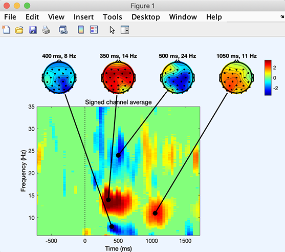
Note that this function may also combine ERSP outputs from different subjects and apply binary statistics.
Plotting measures in scalp topography
Plot time-frequency decomposition
The metaplottopo.m function is a powerful function that allows plotting any measure for all channels and components. For example, the code below allows plotting time-frequency decompositions for all data channels.
eeglab; close; % add path
eeglabp = fileparts(which('eeglab.m'));
EEG = pop_loadset(fullfile(eeglabp, 'sample_data', 'eeglab_data_epochs_ica.set'));
figure; metaplottopo( EEG.data, 'plotfunc', 'newtimef', 'chanlocs', EEG.chanlocs, 'plotargs', ...
                   {EEG.pnts, [EEG.xmin EEG.xmax]*1000, EEG.srate, [0], 'plotitc', 'off', 'ntimesout', 50, 'padratio', 1});

Plot ERP image
Another example below allows plotting ERPimage for all data channels. Note that for ERPimage, the function does not show the axis for each plot making it convenient to plot hundreds of channels if necessary. It is also possible to plot ICA components in this way by replacing EEG.data with EEG.icaact and removing the ‘chanlocs’ argument.
figure; metaplottopo( EEG.data, 'plotfunc', 'erpimage', 'chanlocs', EEG.chanlocs, 'plotargs', ...
         { eeg_getepochevent( EEG, {'rt'},[],'latency') linspace(EEG.xmin*1000, EEG.xmax*1000, EEG.pnts) '' 10 0 });

Creating scalp topography animations
The script used on this page is available at make_eeg_movie.m
Using the eegmovie function to make 2-D scalp topography animations
A simple way to create scalp map animations is to use the (limited)EEGLAB function eegmovie.m from the command line. For instance, to make a movie of the latency range -100 ms to 600 ms, type:
%% Simple 2-D movie
eeglab; close; % add path
eeglabp = fileparts(which('eeglab.m'));
EEG = pop_loadset(fullfile(eeglabp, 'sample_data', 'eeglab_data_epochs_ica.set'));

% Above, convert latencies in ms to data point indices
pnts1 = round(eeg_lat2point(-100/1000, 1, EEG.srate, [EEG.xmin EEG.xmax]));
pnts2 = round(eeg_lat2point( 600/1000, 1, EEG.srate, [EEG.xmin EEG.xmax]));
scalpERP = mean(EEG.data(:,pnts1:pnts2),3);

% Smooth data
for iChan = 1:size(scalpERP,1)
    scalpERP(iChan,:) = conv(scalpERP(iChan,:) ,ones(1,5)/5, 'same');
end

% 2-D movie
figure; [Movie,Colormap] = eegmovie(scalpERP, EEG.srate, EEG.chanlocs, 'framenum', 'off', 'vert', 0, 'startsec', -0.1, 'topoplotopt', {'numcontour' 0});
seemovie(Movie,-5,Colormap);

% save movie
vidObj = VideoWriter('erpmovie2d.mp4', 'MPEG-4');
open(vidObj);
writeVideo(vidObj, Movie);
close(vidObj);
Below, we use the same function to plot the ERP on a 3-D head plot.
Using the eegmovie function to make 3-D scalp topography animations
Run the script above first. The script below creates a 3-D head plot movie.
%% Simple 3-D movie
% Use the graphic interface to coregister your head model with your electrode positions
headplotparams1 = { 'meshfile', 'mheadnew.mat'       , 'transform', [0.664455     -3.39403     -14.2521  -0.00241453     0.015519     -1.55584           11      10.1455           12] };
headplotparams2 = { 'meshfile', 'colin27headmesh.mat', 'transform', [0          -13            0          0.1            0        -1.57         11.7         12.5           12] };
headplotparams  = headplotparams1; % switch here between 1 and 2

% set up the spline file
headplot('setup', EEG.chanlocs, 'STUDY_headplot.spl', headplotparams{:}); close

% check scalp topo and head topo
figure; headplot(scalpERP(:,end-50), 'STUDY_headplot.spl', headplotparams{:}, 'maplimits', 'absmax', 'lighting', 'on');
figure; topoplot(scalpERP(:,end-50), EEG.chanlocs);
figure('color', 'w'); [Movie,Colormap] = eegmovie( scalpERP, EEG.srate, EEG.chanlocs, 'framenum', 'off', 'vert', 0, 'startsec', -0.1, 'mode', '3d', 'headplotopt', { headplotparams{:}, 'material', 'metal'}, 'camerapath', [-127 2 30 0]);
seemovie(Movie,-5,Colormap);

% save movie
vidObj = VideoWriter('erpmovie3d1.mp4', 'MPEG-4');
open(vidObj);
writeVideo(vidObj, Movie);
close(vidObj);
In the script above, change the line “headplotparams = headplotparams1;” to “headplotparams = headplotparams2;” to switch between headmodels.
It is also possible to create frames for movies as shown in the next section.
Creating a movie from frames
Another solution here is to assemble a series of images into a movie. For example, type:
%% Using topoplot to make movie frames
vidObj = VideoWriter('erpmovietopoplot.mp4', 'MPEG-4');
open(vidObj);
counter = 0;
for latency = -100:10:600 %-100 ms to 1000 ms with 10 time steps
    figure; pop_topoplot(EEG,1,latency, 'My movie', [] ,'electrodes', 'off'); % plot'
    currFrame = getframe(gcf);
    writeVideo(vidObj,currFrame);
    close;  % close current figure
end
close(vidObj);