In the previous analysis, at the 1st level, we selected ‘face_type’ (figure 7) as our variable. By doing so, beta parameters reflect the average height of each face type. We know that there is also a repetition effect – and if one repetition differs a lot more than the others that average can be biased. It is therefore recommended to always create a full design (all known effects) and pool conditions to create contrasts.

1st level

For this experiment, we have 9 conditions: familiar faces 1st time, familiar faces 2nd time, familiar faces 3rd time, scrambled faces 1st time, scrambled faces 2nd time, scrambled faces 3rd time, unfamiliar faces 1st time, unfamiliar faces 2nd time, unfamiliar faces 3rd time. We here pool the repetition levels to create only 3 conditions: familiar, scrambled, unfamiliar. The design will be with 6 conditions, but 3 contrasts will also be created – those contrasts are the averages of repetition levels beta parameters (so we expect very similar results, but not identical).

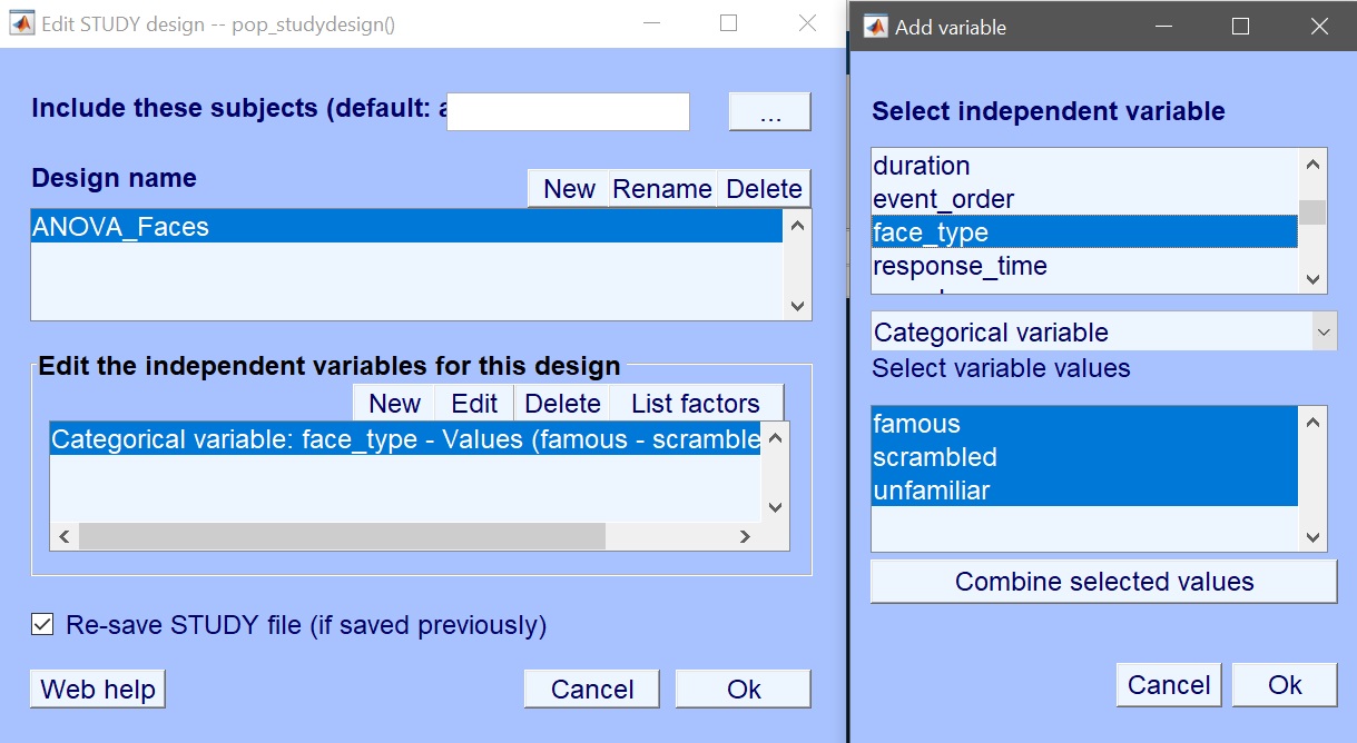
From STUDY, create a new design and let’s call it ‘FaceRepAll’ and then click ‘new’ to add conditions figure 18.

Figure 18. New design pooling conditions

The variable of interest is ‘trial_type’ which contains the 9 experimental conditions. Instead of just selecting those conditions, here let’s combine the repetition levels. Select ‘famous new’, ‘famous second early’ and ‘famous second late’ and click combine selected values (figure 19). Repeat for scrambled and unfamiliar faces. This creates 3 new values (figure 20) which you now select for your design.

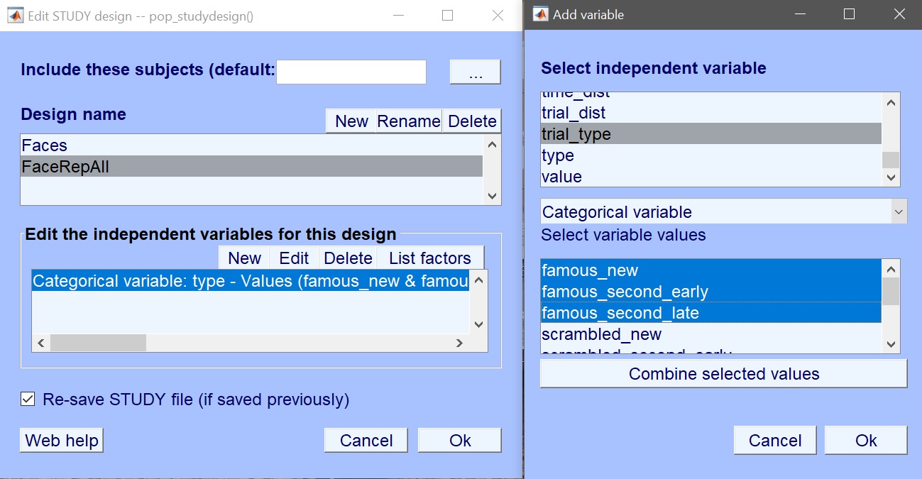Figure 19. New design using trial type

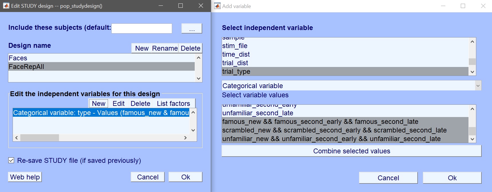Figure 20. Use combined values of trial type

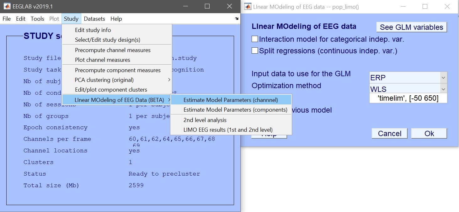
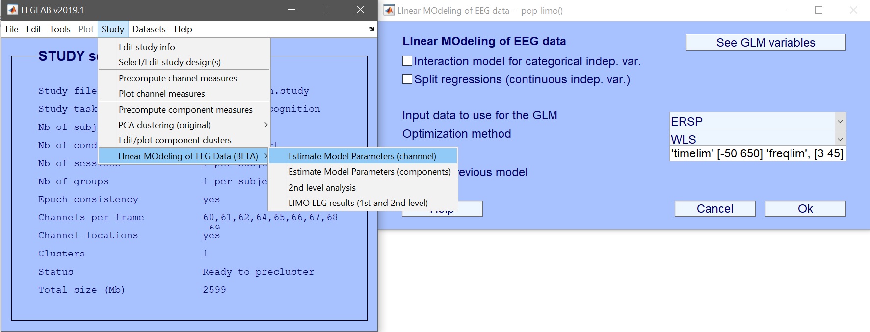
Now estimate model parameters. Input the data type (figure 8 ERP, Spectrum, ERSP) and possibly restrict the time or frequency range. The default method (Weighted Least Squares) is the preferred options, as long as you have more trials than data frames. In addition to the beta parameters, we now have 3 con.mat* files corresponding to the pooled repetition levels.

% 1st level analysis - specify the design
% Note we use the variable 'type' and use cells within a cell array to
% indicate grouping which means contrasts will be computed pooling those levels
STUDY = std_makedesign(STUDY, ALLEEG, 2, 'name','FaceRepAll','delfiles','off','defaultdesign','off',...
    'variable1','type','values1',{{'famous_new','famous_second_early','famous_second_late'},...
    {'scrambled_new','scrambled_second_early','scrambled_second_late'},...
    {'unfamiliar_new','unfamiliar_second_early','unfamiliar_second_late'}},'vartype1','categorical',...
    'subjselect',{'sub-002','sub-003','sub-004','sub-005','sub-006','sub-007','sub-008','sub-009',...
    'sub-010','sub-011','sub-012','sub-013','sub-014','sub-015','sub-016','sub-017','sub-018','sub-019'});
[STUDY, EEG] = pop_savestudy( STUDY, EEG, 'savemode','resave');

% 1st level analysis - estimate parameters
% ERP
[STUDY] = pop_limo(STUDY, ALLEEG, 'method','WLS','measure','daterp','timelim',[-50 650], ...
        'erase','on','splitreg','off','interaction','off');
% Spectrum
[STUDY] = pop_limo(STUDY, ALLEEG, 'method','WLS','measure','daterp','freqlim',[3 45], ...
        'erase','on','splitreg','off','interaction','off');
% ERSP
[STUDY] = pop_limo(STUDY, ALLEEG, 'method','WLS','measure','daterp','timelim',[-50 650],'freqlim',[3 45], ...
        'erase','on','splitreg','off','interaction','off');

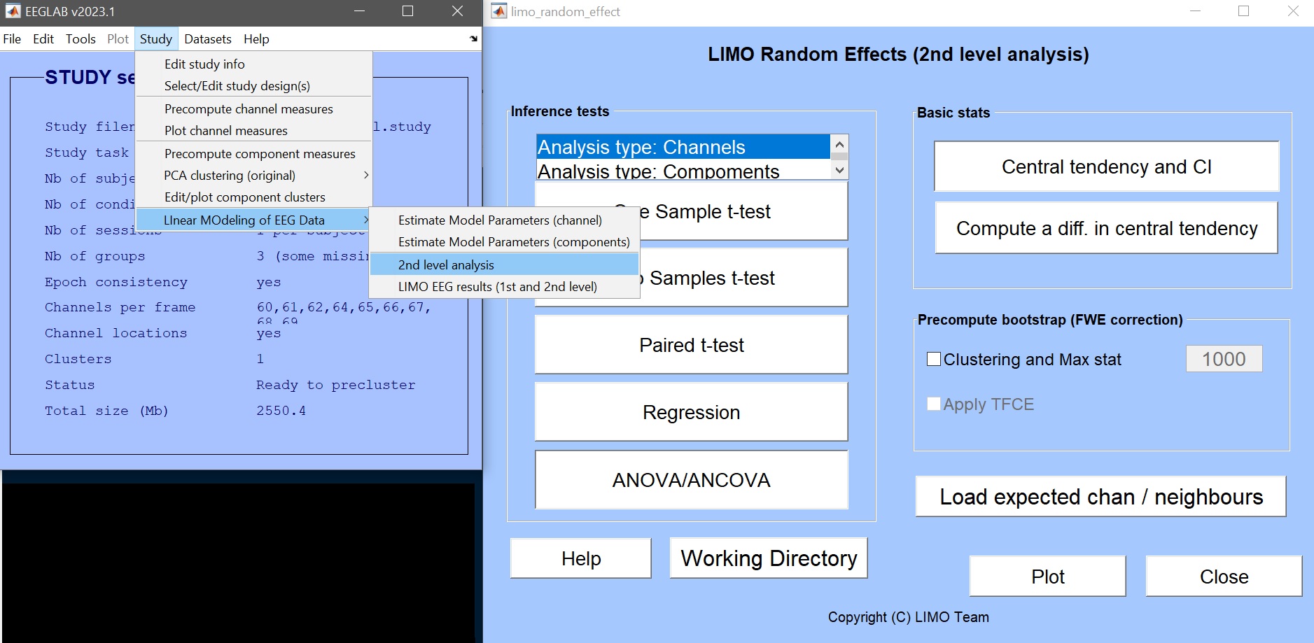
2nd level

Click on Study –> Linear MOdeling of EEG Data –> 2nd level analysis (figure 9).

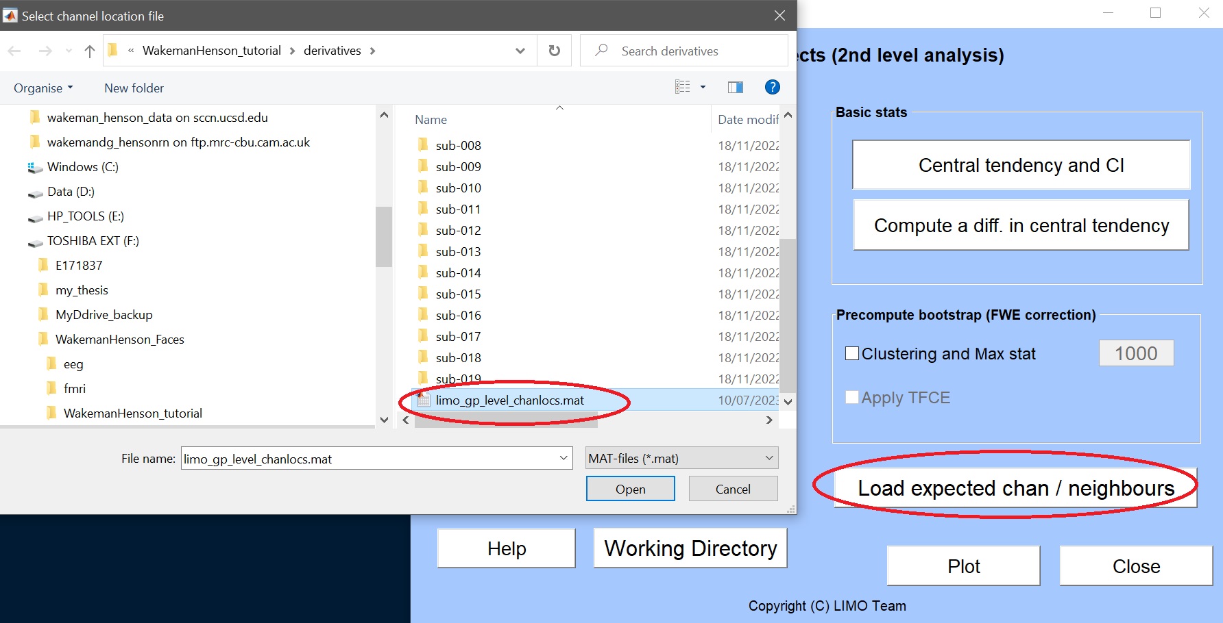
load the group level channel location file – this should be located at the root of the derivatives folder (figure 10)
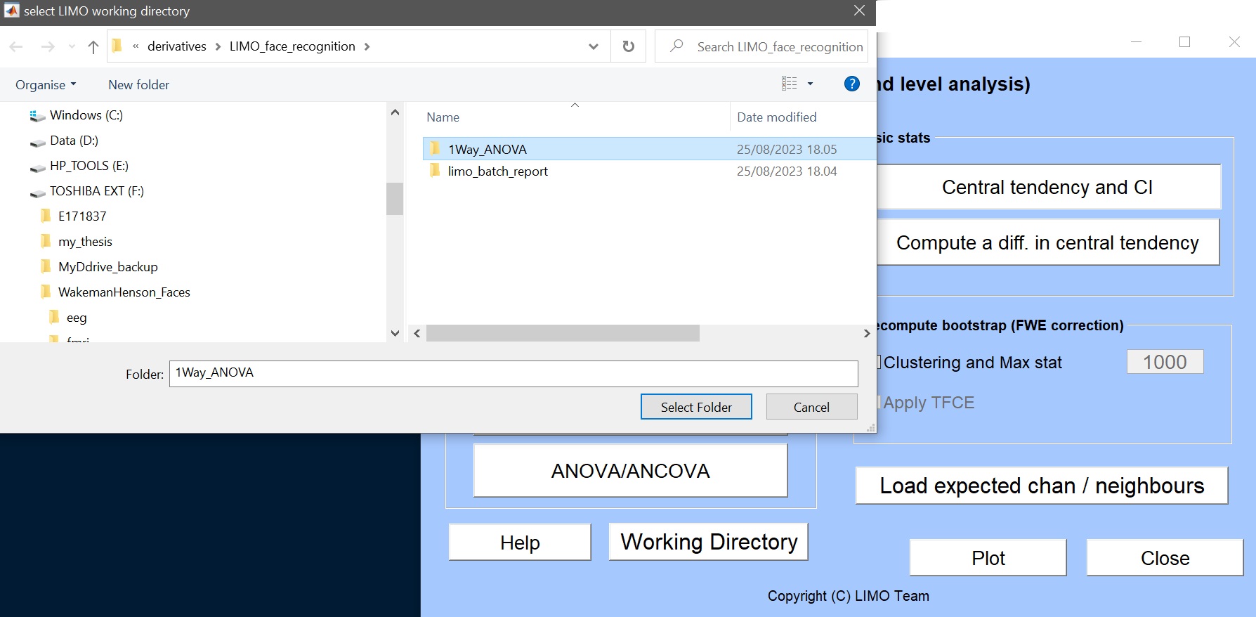
make a new directory (‘1way_ANOVA_revised’) to save this new analysis and select this as a working directory (figure 11)
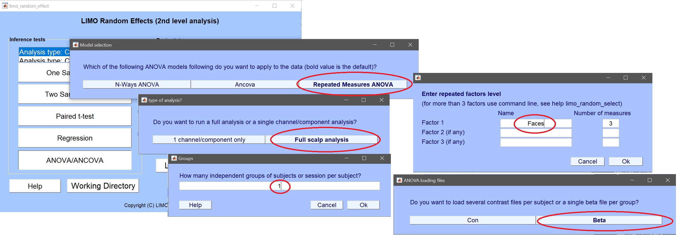
click on ANOVA/ANCOVA (figure 12) and fill the information as needed: Full scalp analysis –> Repeated measure ANOVA –> 1 group –> 1 factor of 3 levels
select con files, iteratively for each level (figure 21), and name that factor ‘faces’

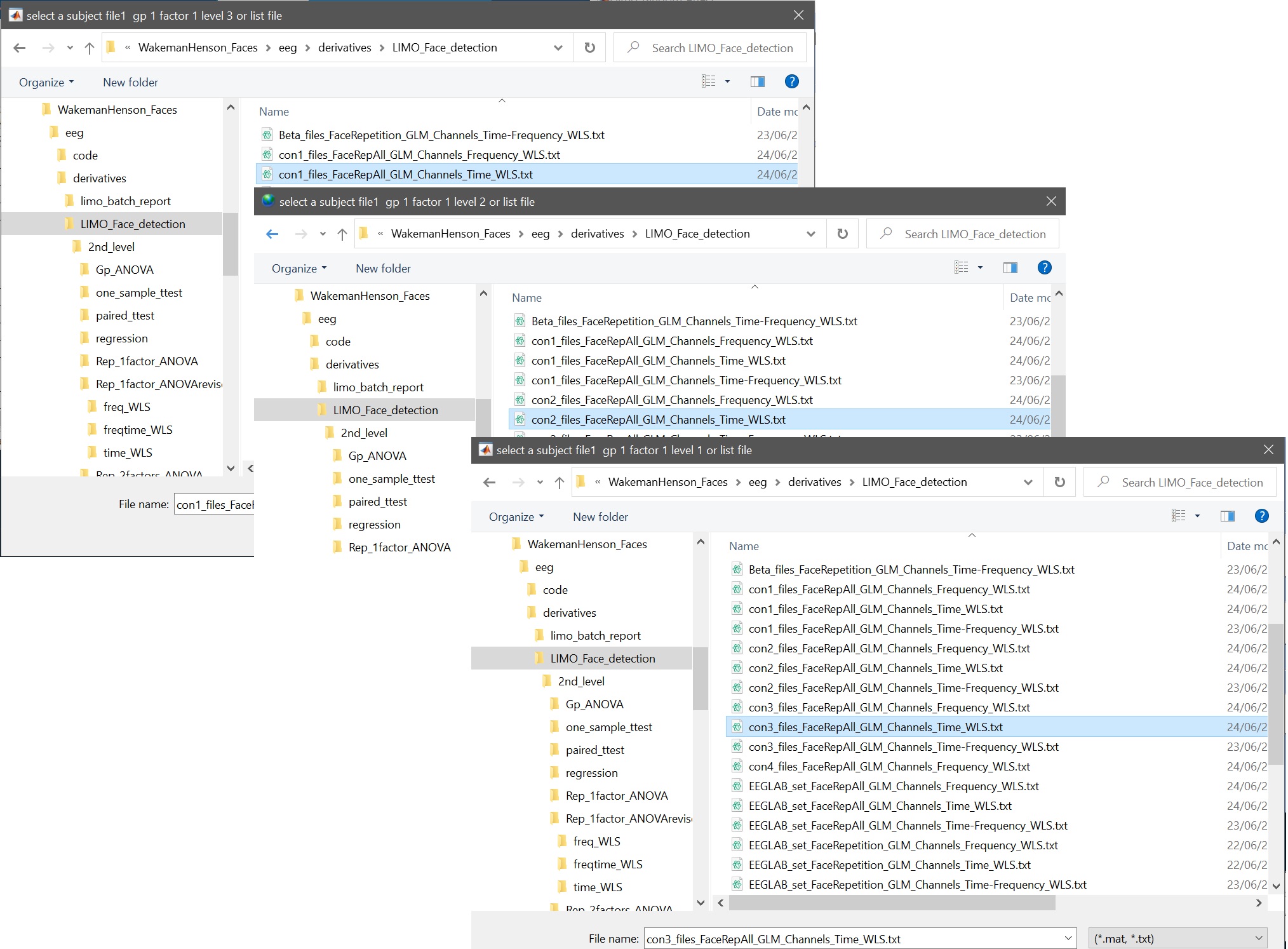Figure 21. Select con files for the ANOVA Figure 21. Select con files (here shown for ERP, i.e. Channels Time WLS) for the ANOVA

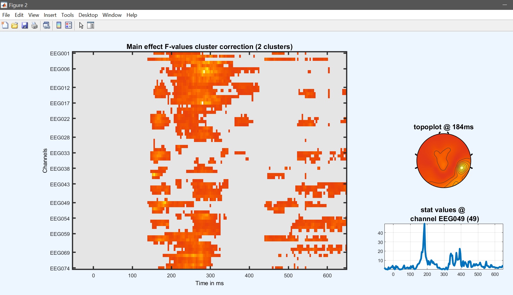
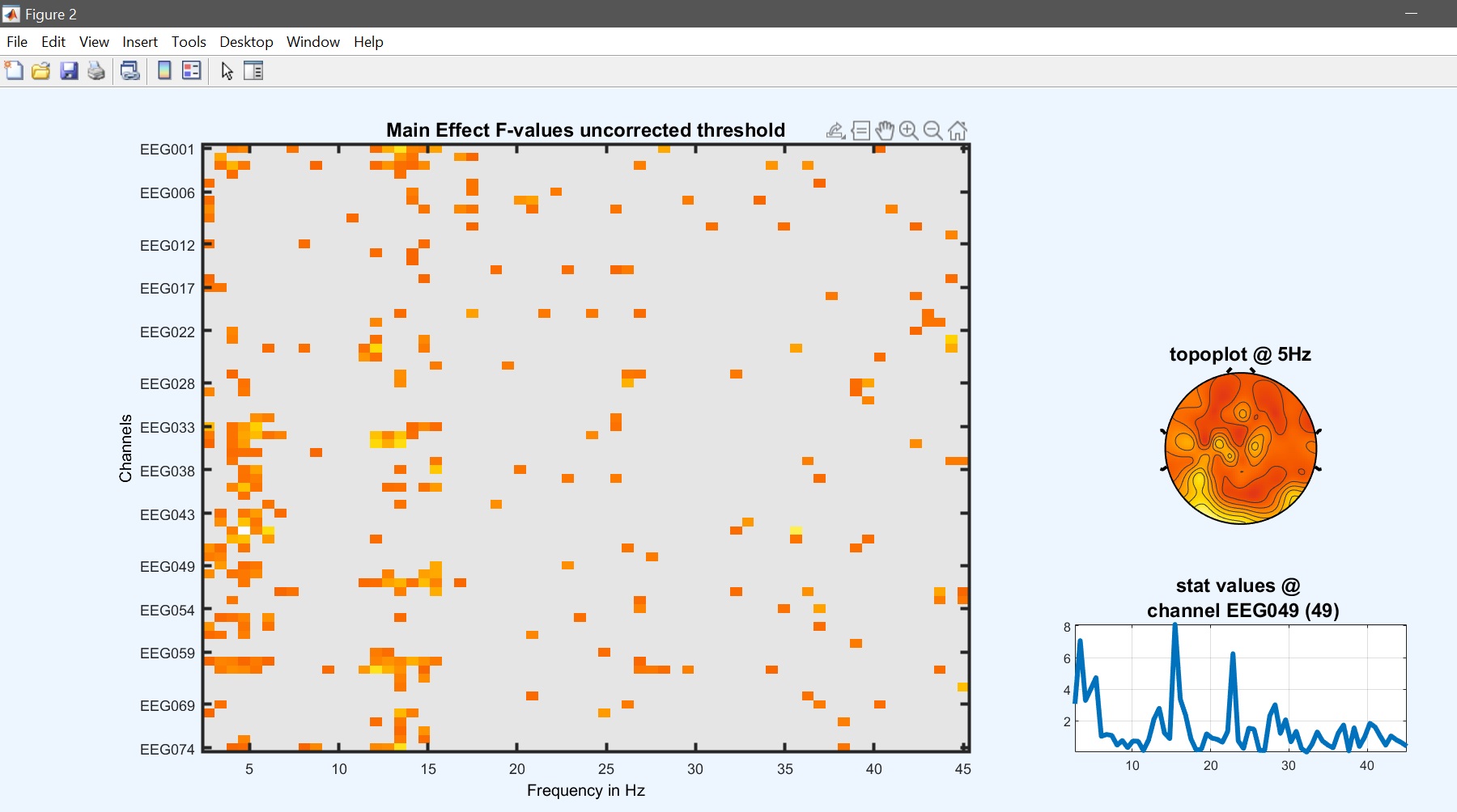
The design matrix should then pop up and answer ‘yes’ to start the analysis. Then review the results (figure 22). While most effects are the same, results differ from figure 15.

Figure 22a. 1-way ANOVA results

chanlocs   = [STUDY.filepath filesep 'limo_gp_level_chanlocs.mat'];
con1_files = fullfile(STUDY.filepath,['LIMO_' STUDY.filename(1:end-6)],'con_1_files_FaceRepAll_GLM_Channels_Time_WLS.txt');
con2_files = fullfile(STUDY.filepath,['LIMO_' STUDY.filename(1:end-6)],'con_2_files_FaceRepAll_GLM_Channels_Time_WLS.txt');
con3_files = fullfile(STUDY.filepath,['LIMO_' STUDY.filename(1:end-6)],'con_3_files_FaceRepAll_GLM_Channels_Time_WLS.txt');

mkdir([STUDY.filepath filesep '1-way-ANOVA-revised'])
cd([STUDY.filepath filesep '1-way-ANOVA-revised'])
limo_random_select('Repeated Measures ANOVA',chanlocs,'LIMOfiles', {con1_files,con2_files,con3_files},...
    'analysis_type','Full scalp analysis','parameters',{[1 1 1]},...
    'factor names',{'face'},'type','Channels','nboot',1000,'tfce',0,'skip design check','yes');

limo_eeg(5,pwd) % channel*time imagesc 

Figure 22b. 1-way ANOVA results

chanlocs   = [STUDY.filepath filesep 'limo_gp_level_chanlocs.mat'];
con1_files = fullfile(STUDY.filepath,['LIMO_' STUDY.filename(1:end-6)],'con_1_files_FaceRepAll_GLM_Channels_Frequency_WLS.txt');
con2_files = fullfile(STUDY.filepath,['LIMO_' STUDY.filename(1:end-6)],'con_2_files_FaceRepAll_GLM_Channels_Frequency_WLS.txt');
con3_files = fullfile(STUDY.filepath,['LIMO_' STUDY.filename(1:end-6)],'con_3_files_FaceRepAll_GLM_Channels_Frequency_WLS.txt');

mkdir([STUDY.filepath filesep '1-way-ANOVA-revised'])
cd([STUDY.filepath filesep '1-way-ANOVA-revised'])
limo_random_select('Repeated Measures ANOVA',chanlocs,'LIMOfiles', {con1_files,con2_files,con3_files},...
    'analysis_type','Full scalp analysis','parameters',{[1 1 1]},...
    'factor names',{'face'},'type','Channels','nboot',1000,'tfce',0,'skip design check','yes');

limo_eeg(5,pwd) % channel*freq imagesc 

Figure 22c. 1-way ANOVA results

chanlocs   = [STUDY.filepath filesep 'limo_gp_level_chanlocs.mat'];
con1_files = fullfile(STUDY.filepath,['LIMO_' STUDY.filename(1:end-6)],'con_1_files_FaceRepAll_GLM_Channels_Time-Frequency_WLS.txt');
con2_files = fullfile(STUDY.filepath,['LIMO_' STUDY.filename(1:end-6)],'con_2_files_FaceRepAll_GLM_Channels_Time-Frequency_WLS.txt');
con3_files = fullfile(STUDY.filepath,['LIMO_' STUDY.filename(1:end-6)],'con_3_files_FaceRepAll_GLM_Channels_Time-Frequency_WLS.txt');

mkdir([STUDY.filepath filesep '1-way-ANOVA-revised'])
cd([STUDY.filepath filesep '1-way-ANOVA-revised'])
limo_random_select('Repeated Measures ANOVA',chanlocs,'LIMOfiles', {con1_files,con2_files,con3_files},...
    'analysis_type','Full scalp analysis','parameters',{[1 1 1]},...
    'factor names',{'face'},'type','Channels','nboot',1000,'tfce',0,'skip design check','yes');

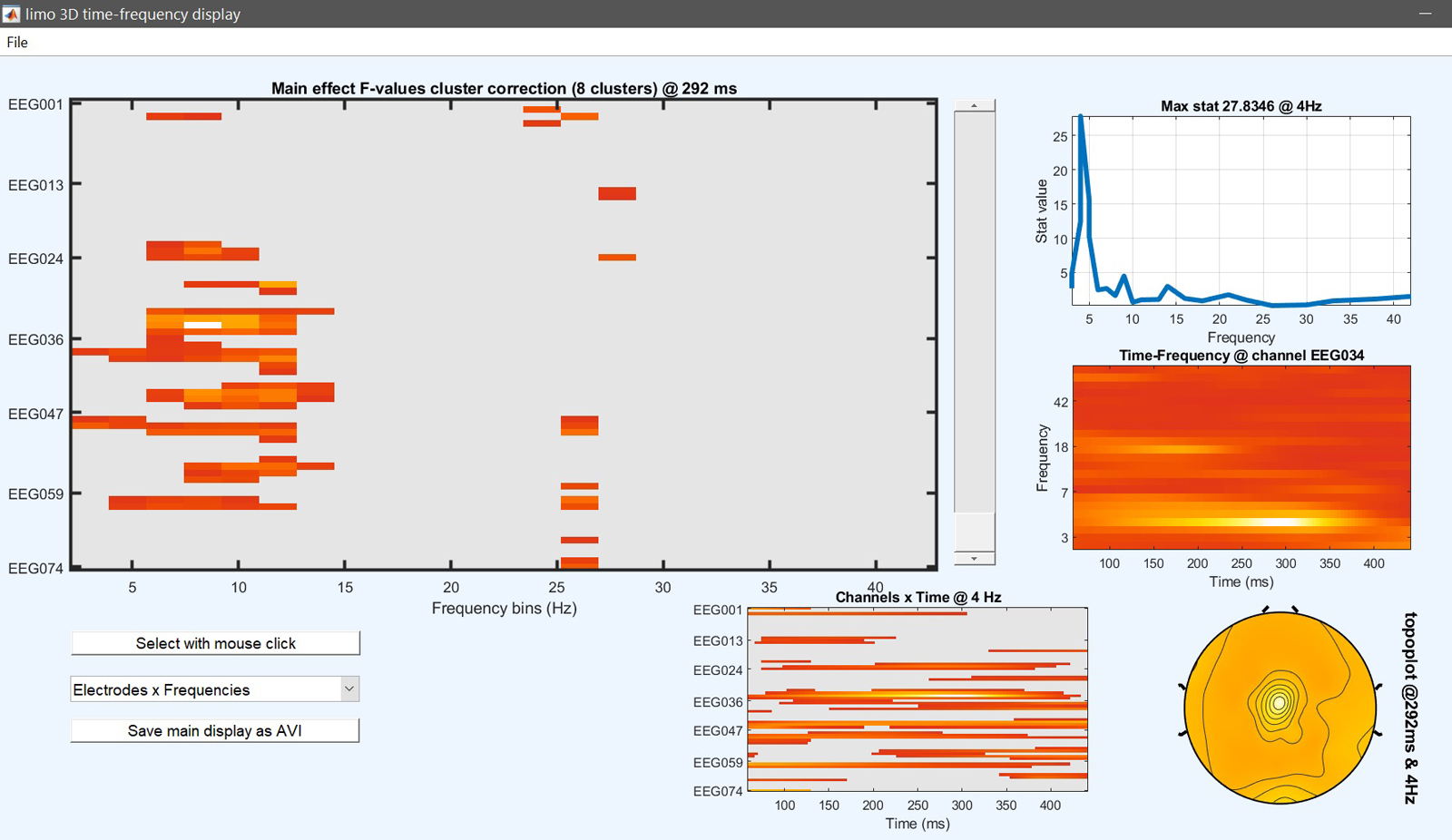
limo_eeg(5,pwd) % channel*time*freq 'imagesc' like 

Figure 22. 1-way ANOVA results based on 1st level contrasts