Precomputing and visualizing channel data
EEGLAB allows plotting grand-average ERPs, spectra, ERPimage, and ERSP/ITCs. In this section of the tutorial, we will see how to pre-compute measures, how to plot them, and how to modify plotting parameters.
Table of contents
Load the sample EEGLAB STUDY set
In each tutorial, we try to illustrate EEGLAB features with different data. In this one, we will use a 14-subject animal/non-animal categorization task.
Subjects were presented with pictures that either contained or did not contain animal images. Subjects responded with a button press whenever the picture presented contained an animal (go/no-go paradigm). These data are available for download here (626 Mb). A complete description of the task, the raw data (4Gb), and some MATLAB files to process it are all available on openneuro.org.
Select menu item File and press sub-menu item Load existing study. Select the tutorial file “animal.study” then press Open.
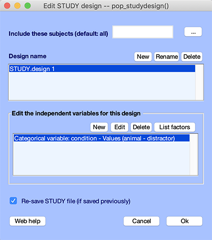
After loading the data, to review the STUDY design, use the Study → Select/Edit study design menu item. The default design is to compare images containing animals with images containing distractors. Press Ok to close the window.
Precomputing and plotting ERPs
Precomputing ERPs
Before plotting the channel measures, you must precompute them using the Study → Precompute channel measures menu item, as shown below.
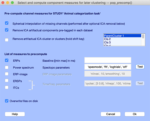
This GUI is divided into two parts, the top part, which specifies transformation to apply to the data before precomputing measures, and the second part, which specifies which measures to precompute.
You may specify channel transformations in the GUI top panel.
-
Channel interpolation. It is highly recommended that for visualizing and computing statistics on data channels, you first interpolate missing channels. Automated interpolation in EEGLAB is based on channel labels. If datasets have different channel locations (for instance, if the locations of the channels were scanned), you must interpolate missing channels for each dataset from the command line using eeg_interp.m. Please select this option.
-
Subtracting artifactual ICA components. This can either be done by removing components tagged for rejection as explained in the tutorial section on using Independent Component Analysis for artifact removal. This requires that you tag components in each dataset (you may also tag components at the STUDY level using the IClabel plugin as explained here). We recommend selecting this option.
-
Subtracting ICA component clusters. Alternatively to using the option above, you may select ICA component clusters to subtract from the data using the third checkbox. Refer to the clustering tutorial for more information.
The bottom panel contains the list of measures to precompute. Tick the box and complete the parameters for the measure(s) you are interested in. For now, let’s select ERPs as it is fast to compute. This computes the mean event-related potential for each condition and electrode. You may specify the baseline you wish to use (leave as blank). Then press Ok.
Change in EEGLAB 2019 and later versions: In EEGLAB 2019 and later versions, EEGLAB directly processes single trials and there is no need to recompute measures for each design, as this was the case with previous EEGLAB versions. The new design scheme is backward compatible, more flexible, and allows extracting data trial measures dynamically.
Plotting grand-average ERPs
After precomputing the channel measures, you may now plot them, using the Study → Plot channel measures menu item.
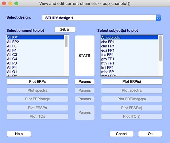
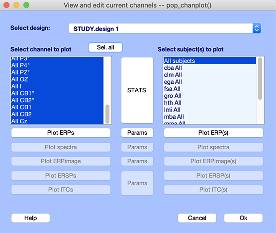
All the measures described in the previous section, once computed, may be used for channel data visualization. Press the Plot ERPs button.
Now, let’s look at the plotting parameters. In the central column of the pop_chanplot.m GUI, you may change plotting parameters using the Params button next to the measure you wish to plot. Press the Params button next to the Plot ERPs button. The following GUI pops up.
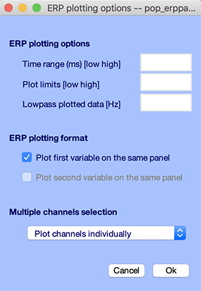
This GUI contains several sections and lets you specify the time range for plotting ERPs and plot limits in microvolt. Please select the checkbox to overlay the two conditions on the same panel as shown above.
There are more options in this GUI. They should be self-explanatory:
- The Time range to plot edit box allows plotting a shorter time range than the full epoch.
- The Plot limits edit box allows setting fixed lower and upper limits to the plotted potentials.
- The Display filter edit box allows entering a frequency (for instance 20 Hz) to filter the ERP. This is only applied to the ERP display and does not affect the computation of statistics. This option is useful when plotting noisy ERPs for single subjects.
In the bottom Multiple channels selection section, you have the choice of:
- Plotting individual channels. The default option.
- Plotting the average topography over a time range (specified in the top box). We will be using this option later in this tutorial.
- Plotting the ERP measure averaged over a subset of channels.
- Compute the root mean square (RMS) of the selected channels - this is equivalent to computing the Global Field Power (GFP).
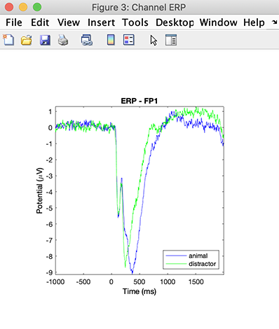
Press Ok and press the Plot ERPs button again. Now the ERPs for the two conditions are plotted together, making it easier to spot differences between them.
Plotting single subject ERPs
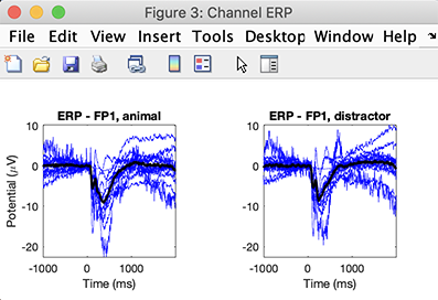
You may plot all subjects’ ERPs by pressing the Plot ERPs pushbutton in the right column, obtaining a figure similar to the one below.
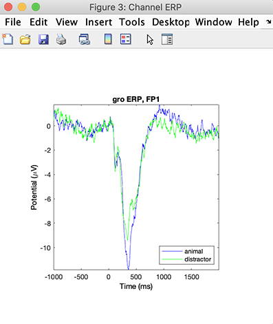
To plot data for a single subject, press the Plot ERPs pushbutton on the right column for subject gro. A plot like the one below should appear. This is useful for reviewing an individual subject’s ERPs.
Plotting all channel ERPs
Finally, you may also plot all scalp channels simultaneously. To do this, click the push button Sel. all to select all data channels.
Then again, press the Plot ERPs button in the left column.
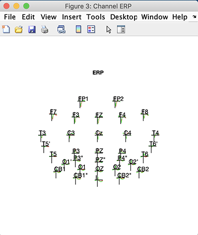
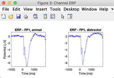
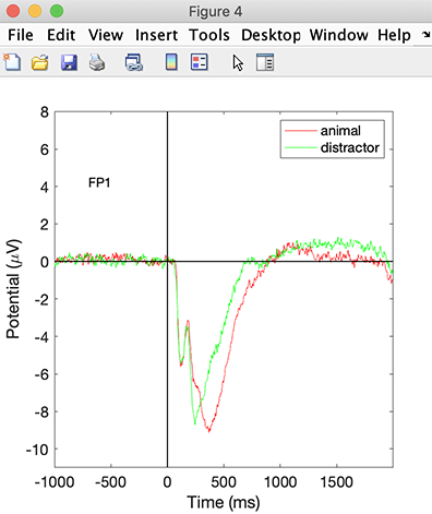
Clicking on individual ERPs will make a window plotting the selected channel ERP pop up. For example, click on channel FP1.
Plotting ERP scalp topographies
In the central column, press the Params button again. Enter the time range “300 400” in the Time range edit box. In the bottom section, select Plot average topography over time range. Then press Ok.
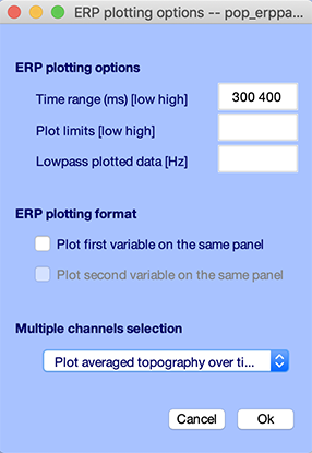
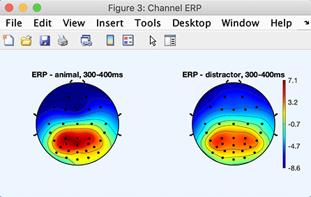
Press the Plot ERPs button again to plot the scalp topographies for the average ERP between 300 and 400 ms. We can see a difference of potential between the two conditions in the parieto-central region, although we would need to run statistics to assess this difference is significant.
Plotting other measures
Precomputing other measures
In addition to ERPs, below is the full list of measures you can compute:
-
Power spectra: performs spectral decomposition for each condition and electrode. You can enter here specific parameters for the spectopo.m function.
-
ERP-image: pre-computes ERP-images.
-
ERPs/ ITCs: allows computing event-related spectral perturbation in the form of event-related spectral power changes (ERSPs), and event-related phase consistencies (ITCs) for each condition. Several time/frequency parameters are required to compute the ERSP and/or ITC measures. To choose these values, you may enter the relevant newtimef.m keywords and arguments in the text box.
-
You may also compute custom measures when calling the pop_precomp.m function from the line, as explained in the group analysis scripting tutorial.
Select the Study → Precompute measures menu item. Tick the box and complete the parameters for all measures. Also, for the ERSP parameters, change the parameters nfreqs to 30 and ntimesout to 60 to speed up calculation, as shown below. Press Ok.
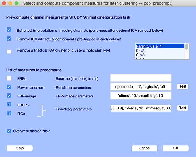
In general, we recommend selecting all measures when possible. Computing spectra and ERP-image is fast and should only take a few seconds. Computing ERSP and ITC should take from two to five minutes. Then again, select the Study → Plot channel measures menu item. All measures are now available for plotting.
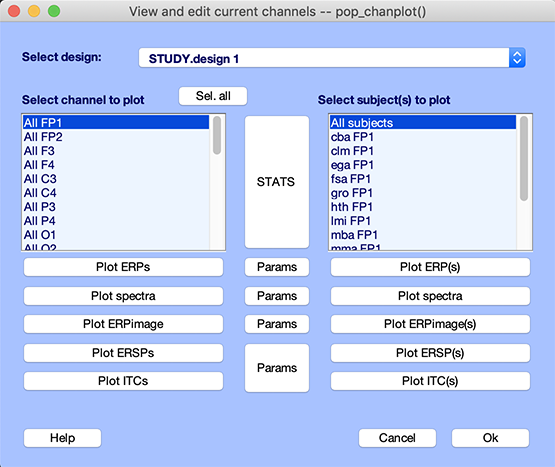
Note that the spectra, ERPimage, and ERSP/ITCs plotting options are similar to the ERP plotting options we looked at previously. For spectra, the menu is similar to the ERP’s menu, with the difference that the top box lets you specify the frequency range you wish to plot. For ERSPs / ITCs, you can specify and time and frequency range as well as power and ITC limits.
Plotting spectra
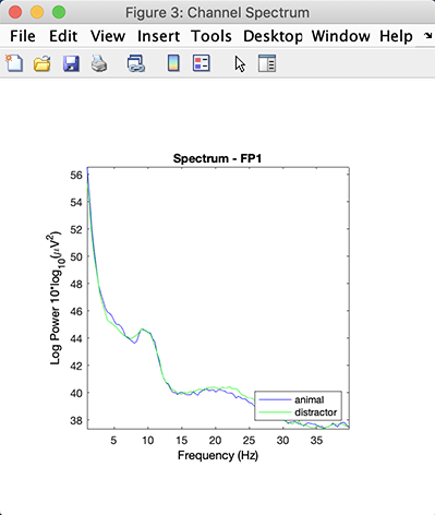
Spectra are plotted in the same way as ERPs are. Let’s first click on the Params button adjacent to the Plot spectra buttons and enter “1 40” for the frequency range. Press Ok.
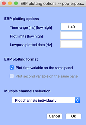
Select the first channel FP1 and press Plot spectra in the left column of the pop_chanplot.m GUI. The following plot pops up.
Plotting ERP image
Press the Plot ERPimage button.
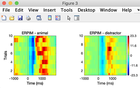
ERP images are plotted with parameters set when pre-computing measures. In particular, we set to use 10 rows. Setting a fixed number of rows allow obtaining matrices of the same size for all subjects and conditions and performing standard statistics as described in Delorme et al. (2014).
Plotting ERSPs and ITCs
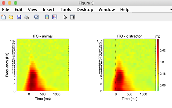
Press the Plot ITC button. This shows inter-trial coherence for the animal and distractor conditions. It appears that the ITC values are of lower amplitude for the distractor condition, although we would need to run statistics to confirm that observation.
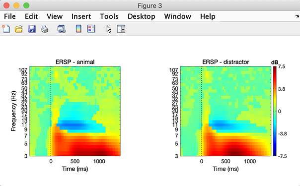
Select channel Oz and press the Plot ERSPs button. The following plot pops up. It shows an increase in power at low frequencies (below 7 Hz) and a decrease in power at about 10 Hz.
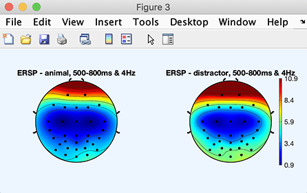
As for ERPs and spectra, it is possible to plot scalp topographies in specific time and frequency ranges. Let’s select the Params button adjacent to the Plot ERSP buttons and enter “500 800” for the time range and 4 for the frequency range. Press Ok.
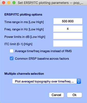
Now press the Plot ERSPs button. The following scalp topographies are shown. It appears that spectral power is lower in the distractor than the animal condition. Again, we would need to run statistics to confirm this observation.
Comparing different sets of pre-compute parameters
Using multiple STUDIES may also be useful for testing different signal processing options. For instance, one might create two identical STUDIES, in one computing the time/frequency measures using FFTs in one and using wavelets in the other one. However, there can only be one set of pre-computed data files associated with the subjects’ data. If you want to compare side by side different sets of pre-compute parameters, you should duplicate the STUDY folder and all associated data files. Saving a second STUDY using a different file name is not sufficient.