Clustering ICA components
This part of the tutorial will demonstrate how to use EEGLAB to interactively preprocess, cluster, and then visualize the dynamics of ICA (or other linear) signal components across one or many subjects by operating on one of the tutorial STUDY.
Table of contents
Why cluster ICA components?
Is my Cz your Cz?
To compare electrophysiological results across subjects, the usual practice of most researchers has been to identify scalp channels (for instance, considering recorded channel Cz in every subject’s data to be spatially equivalent). Actually, this is an idealization, since the spatial relationship of any physical electrode site (for instance, Cz, the vertex in the International 10-20 System electrode labeling convention) to the underlying cortical areas that generate the activities summed by the (Cz) channel may be rather different in different subjects, depending on the physical locations, extents, and particularly the orientations of the cortical source areas, both in relation to the ‘active’ electrode site (e.g., Cz) and/or to its recorded reference channel (for example, the nose, right mastoid, or other sites).
That is, data recorded from equivalent channel locations (Cz) in different subjects may sum the activity of different mixtures of underlying cortical EEG sources, no matter how accurately the equivalent electrode locations were measured on the scalp. This fact is commonly ignored in EEG research.
Is my IC your IC?
Following ICA (or other linear) decomposition, however, there is no natural and easy way to identify a component from one subject with one (or more) component(s) from another subject. A pair of independent components (ICs) from two subjects might resemble and/or differ from each other in many ways and to different degrees – by differences in their scalp maps, power spectra, ERPs, ERSPs, ITCs, or etc. Thus, there are many possible (distance) measures of similarity and many different ways of combining activity measures into a global distance measure to estimate component pair similarity.
Thus, the problem of identifying equivalent components across subjects is non-trivial. EEGLAB contains functions and supporting structures for flexibly and efficiently performing and evaluating component clustering across subjects and conditions (see 2004 and 2005). With its supporting data structures and stand-alone std_ prefix analysis functions, EEGLAB makes it possible to summarize results of ICA-based analysis across more than one condition from a large number of subjects. This makes more routine use of linear decomposition and ICA possible to apply to a wide variety of hypothesis testing on datasets from several to many subjects.
Note that independent component clustering (like much other data clustering) has no single correct solution. Interpreting the results of component clustering, therefore, warrants caution. Claims to the discovery of physiological facts from component clustering should be accompanied by thoughtful caveat and, preferably, by results of statistical testing against suitable null hypotheses.
Prepare data for ICA component clustering
Load and prepare data
In this tutorial, we will use a 5-subject STUDY (450Mb). See the STUDY creation tutorial for more information on this data. Select menu item File and press sub-menu item Load existing study. Select the tutorial file “N400.study” then press Open.
The STUDY above is ready for clustering, but the following steps are usually required before clustering ICA components.
- You have created a STUDY with the data from all participants in your experiment. See STUDY creation tutorial.
- You have added channel locations. Note that channel locations may be edited for all datasets at the same time (simply use menu item Edit → Channel locations).
- You have run ICA on each dataset. Use menu item Tools → Decompose data by ICA to run ICA on all datasets if this is not the case.
- You have fitted each ICA component with a dipole. If this is not the case, use menu item Tools → Locate dipoles using DIPFIT -> Head model and settings, and then Tools → Locate dipoles using DIPFIT -> Autofit.
- You have regularly saved your changes using menu item File → Save current study. You can save the updated STUDY set to disk, either overwriting the current version - by leaving the default file name in the text box - or by entering a new file name.
Select components to cluster
Then select the menu item Study → Edit study info. The following interface pops up.
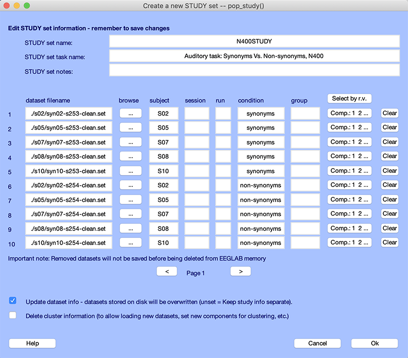
We have already described this interface when importing data in a STUDY in the STUDY creation tutorial. The bottom checkbox removes all current cluster information, and you need to check this checkbox if you want to remove all clusters or if you have added or removed datasets (because the modified STUDY would not be consistent with the already computed clusters). The button Select by r.v. allows you to set a threshold for residual variance of the dipole model associated with each component. Press this button. The entry box below will appear.
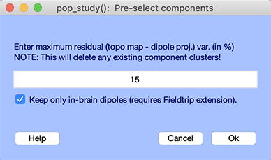
This interface allows specifying that components used in clustering will only be those whose equivalent dipole models have residual dipole variance of their component map, compared to the best-fitting equivalent dipole model projection to the scalp electrodes, less than a specified threshold (0% to 100%). The default r.v. value is 15%, meaning that only components with dipole models’ residual variance of less than 15% will be included in clusters. This is useful because of the modeled association between components with near dipolar (or sometimes dual-dipolar) scalp maps with physiologically plausible components, those that may represent the activation in one (or two coupled) brain area(s). For instance, in the interface above, the default residual variance threshold is set to 15%. This means that only components that have equivalent dipole models with less than 15% of residual variance will be selected for clustering (see this article for a justification of the 15% threshold). Pressing Ok will cause the component column to be updated in the main study-editing window.
The Comp. buttons contains the components for each dataset that will be clustered based on the residual variance threshold selected above. You may edit these manually. Note that if you change the component selection (by pressing the relevant push button), all datasets with the same subject name and the same session number will also be updated (as these datasets have the same ICA decompositions).
Press Ok in the STUDY editing GUI to save your changes.
Multiple ICA decompositions per subject
Continuous data collected in one task or experiment session are often separated into epochs defining different task conditions (for example, separate sets of epochs time-locked to targets and non-targets, respectively). Datasets from different conditions collected in the same session are assumed by the clustering functions to have the same ICA component weights (i.e., the same ICA decomposition is assumed to have been applied to the data from all session conditions at once). If this was not the case, then datasets from the different conditions must be assigned to different sessions.
So, we recommend performing one ICA decomposition on all the data collected in each data collection session, even when several conditions are involved. In our experience, ICA can return a more stable decomposition when trained on more data. Having components with common spatial maps also makes it easier to compare component behaviors across conditions. To use the same ICA decomposition for several conditions, simply run ICA on the continuous or epoched data before extracting separate datasets corresponding to specific task conditions of interest. Then extract specific condition datasets; they will automatically inherit the same ICA decomposition. We followed this procedure for the tutorial data used on this page.
Compute component activity measures
The next step before clustering is to precompute component activity measures for each dataset. Precomputing measure is necessary to cluster components but it is also necessary to visualize component activities. Note that the GUI for precomputing component activity measures is similar to the GUI for precomputing channel activity described in the channel visualization tutorial.
Select menu item Study → Precompute component measures. In the interface below, select all measures. For ERSP/ITC, select 30 frequencies and 60 time points to speed up computation, as shown below. Press Ok.
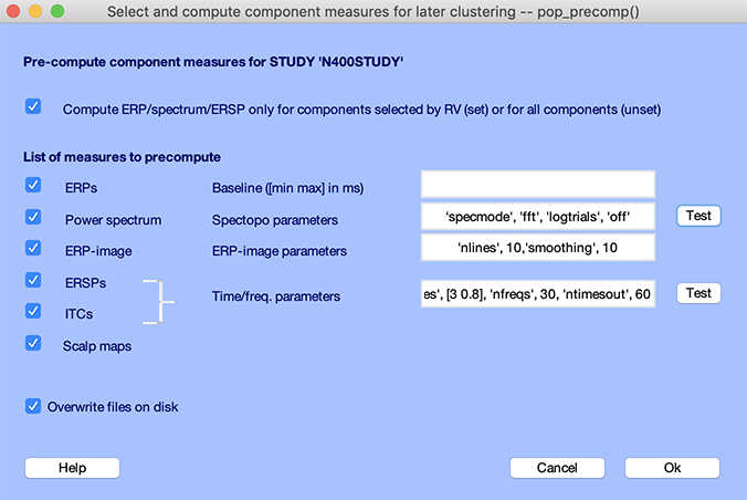
It should take a few minutes to precompute all measures.
Cluster components
The main method to cluster components in EEGLAB is the PCA clustering method described below. Other methods are the Measure Projection method and the Scalp Correlation method available in EEGLAB plugins as indicated in a subsequent section.
Building a preclustering matrix
The aim of the preclustering interface is to build a global distance matrix specifying distances between components for use by the clustering algorithm. This component distance is typically abstract, estimating how far the components’ maps, dipole models, and/or activity measures are from one another in the space of the joint, PCA-reduced measures selected. This will become clearer as we detail the use of the graphic interface below.
The condition means used to construct this overall cluster distance measure may be selected from a palette of standard EEGLAB measures: ERP, power spectrum, ERSP, and/or ITC, as well as the component scalp maps (interpolated to a standard scalp grid) and their equivalent dipole model locations. Note that dipole locations are the one type of preclustering information not precomputed since it is readilly available in each dataset.
Invoke the preclustering graphic interface (pop_preclust.m function) by using menu item Study → PCA clustering (original) → Build preclustering array function and its GUI interface described below first computes desired condition-mean measures used to determine the cluster distance of components from each other.
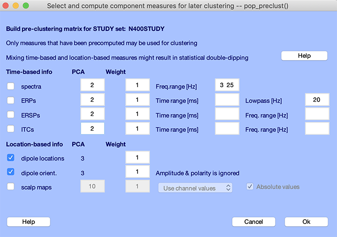
The checkboxes on the left in the second section of the pop_preclust.m interface above allow selection of the component activity measures to include in the cluster location measure constructed to perform clustering.
The goal of the preclustering function is to compute an N-dimensional cluster position vector for each component. These cluster position vectors will be used to measure the distance of components from each other in the N-dimensional cluster space. The N-dimensional vector incorporates information from PCA-reduced ERP, ERSP, or other measures. The value of N is arbitrary but, because of constraints imposed by clustering algorithms, should be kept relatively low (about 10, e.g., <3 or less per measure).
In the cluster position vectors, for example, the three first values might represent the 3-D (x, y, z) spatial locations of the equivalent dipole for each component. The next, say, 2 values might represent the largest 2 principal components of the first condition ERP, the next 2, for the second condition ERP, and so on. If you are computing (time/frequency) spectral perturbation images, you cannot use all their (near-3000) time-frequency values. Here also, you should use the Dim. column inputs to reduce the number of dimensions (for instance, to 2 or 3).
Dimension normalization
You may wish to normalize these principal dimensions for the location and activity measures you select so their metrics are equivariant across measures. Do this by checking the checkbox under the norm column. This normalization process involves dividing the measure data of all principal components by the standard deviation of the first PCA component for this measure.
You may also specify a relative weight (versus other measures). For instance, if you use two measures (A and B) and you want A to have twice the”weight of B, you would normalize both measures and enter a weight of 2 for A and 1 for B. If you estimate that measure A has more relevant information than measure B, you could also enter a greater number of PCA dimension for A than for B.
Component measures
All the measures described below, once computed, can be used for clustering and/or for cluster visualization. First, we have the time-based measures.
-
Spectra: The first checkbox allows you to include the log mean power spectrum for each condition in the preclustering measures. Clicking on the checkbox allow you to enter power spectral parameters. In this case, a frequency range [lo hi] (in Hz) is required. Note that for clustering purposes (but not for display), for each subject individually, the mean spectral value (averaged across all selected frequencies) is subtracted from all selected components, and the mean spectral value at each frequency (averaged across all selected components) is subtracted from all components. The reason is that some subjects have larger EEG power than others. If we did not subtract the (log) means, clusters might contain components from only one subject, or from one type of subject (e.g., men, who often have thinner skulls and therefore larger EEG than women).
-
ERPs: The second checkbox computes mean ERPs for each condition. Here, an ERP latency window [lo hi] (in ms) is required.
-
ERSPs and/or ITCs: The following two checkboxes allow including event-related spectral perturbation information in the form of event-related spectral power changes (ERSPs), and event-related phase consistencies (ITCs) for each condition.
Second, we have the location-based measures.
-
Dipole locations: The third checkbox allows you to include component equivalent dipole locations in the preclustering process. Dipole locations (shown as [x y z]) automatically have three dimensions. It is also possible to cluster on dipole orientations. As mentioned before, the equivalent dipole model for each component and dataset must already have been precomputed. If one component is modeled using two symmetrical dipoles, the pop_preclust.m function will use the average location of the two dipoles for clustering.
-
Scalp maps: The last checkbox allows you to include scalp map information in the component cluster location. You may choose to use raw component map values, their laplacians, or their spatial gradients. We have obtained fair results for main components using laplacian scalp maps, though there are still better reasons to use equivalent dipole locations instead of scalp maps. You may also select whether or not to use only the absolute map values, their advantage being that they do not depend on (arbitrary) component map polarity. We do not recommend to use dipole and scalp map information as the information is redundant.
In the pop_preclust.m interface shown above, select only the dipole checkboxes and leave all default parameters (including the dipole residual variance filter at the top of the window). The total number of dimension is the sum of the dimension for all selected measures (in our case, 3+3 = 6). Clustering algorithms may not work well with more than 10 dimensions, especially if the number of components is limited. In our case, the number of dimensions (6) compared to the number of components (151, elected based on residual variable threshold) is acceptable.
Press Ok.
Applying the clustering algorithm
You may call the pop_clust.m cluster function interface by selecting the Study → PCA clustering (original) → Cluster components menu item, as shown below.
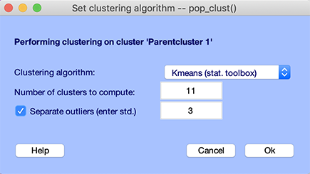
Several algorithms are available: kmeans, neural network, affinity, and affinity clustering.
Kmeans requires the MATLAB Statistics Toolbox, while neural network clustering uses a function from the MATLAB Neural Network Toolbox. A version of kmeans that does not require the MATLAB Statistics Toolbox is also available. Affinity clustering does not require any toolbox. We recommend using affinity clustering which does not require to specify the number of clusters, then try the kmeans algorithm if the results are not satisfactory.
For kmeans, note that the default number of clusters is set so on average there will be one computed per subject per cluster. For example, if about 20 components per subjects are selected based on the residual variance threshold and the STUDY contains 10 subjects, the average number of cluster will be set to 20 - so each cluster will contains on average 10 components. In this case, we have a reduced number of subject, so enter 11 to increase the number of component per cluster.
An option for the kmeans.m algorithm can relegate outlier components to a separate cluster. Outlier components are defined as components further than a specified number of standard deviations (3, by default) from any of the cluster centroids. To turn on this option, click the upper checkbox on the left. Identified outlier components will be placed into a designated Outliers cluster (Cluster 2).
Press Ok. The cluster editing interface detailed in one of the following sections will automatically pop up.
Optimal Kmeans clustering
We have recently added Optimal Kmeans algorithm to the pop_clust function. This feature allows you to find the optimal number of clusters for your data. To use this feature, you must have the MATLAB Statistics and Machine Learning Toolbox installed.
To use this feature, select the Optimal Kmeans option from the Clustering algorithm dropdown menu. Then, you need to input a range of cluster numbers to test (in the screenshot below, the minimum is set to 10, and the maximum is set to 30). The algorithm will then test the clustering for each number of clusters in the range and choose the optimal number of clusters based on the silhouette score. The silhouette score is a measure of how similar an object is to its own cluster compared to other clusters. The optimal number of clusters is the one that maximizes the silhouette score. Read more about the silhouette score from the MATLAB documentation.
Recommended number of clusters: Following the rationale for the estimated number of clusters above, we recommend setting the lower bound of the cluster range to half the average number of components per subject. For example, if there are 20 components per subject, set the lower bound to 10. Similarly, set the upper bound to 1.5 times the average number of components per subject. For example, for 20 components per subject, set the upper bound to 30. If the returned number of clusters is at its lower or upper bound, consider expanding the range. We also strongly recommend using the option to separate outliers.

Other clustering methods
The main method to cluster components in EEGLAB is the PCA clustering method described in this tutorial. Other methods are the Measure Projection method and the Scalp Correlation method available in the EEGLAB plugins described below.
Finding clusters with the Measure Projection plugin
Using measure projection, IC measures (ERP, ERSP…, except equivalent dipoles), are compared for each IC pair and their dissimilarity is multiplied to form a combined pairwise dissimilarity matrix. This matrix is then normalized, weighted, and added to the normalized and weighted IC equivalent dipole distance matrix. The final dissimilarity matrix is then clustered using affinity clustering method. Refer to the plugin GitHub repository for details.
Finding clusters with the Corrmap plugin
Corrmap is an EEGLAB plugin that clusters components based on the correlation of their scalp topographies. The documentation for this plugin is available on Stefan Debener web page and the plugin GitHub repository.
Visualizing component clusters
Call the cluster editing function pop_clustedit.m using menu item Study → Edit → plot clusters. This will open the following window.
Note that the clustering menu item Study → PCA clustering (original) → Cluster components we used in a previous section will also call automatically this window after clustering has finished.
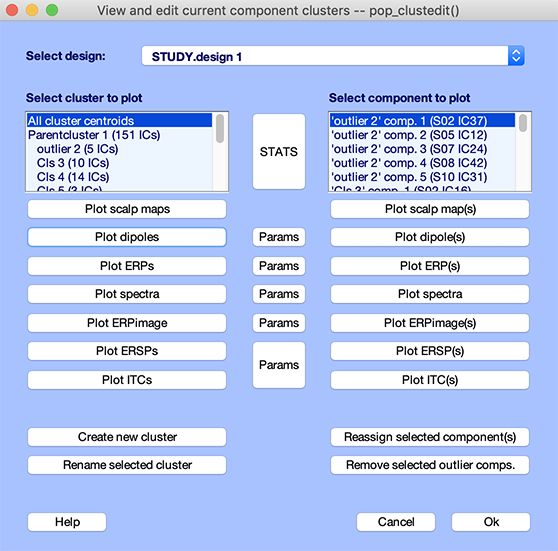
Of the 305 components in the sample N400 STUDY, dipole model residual variances for 151 components were below 15%. Other components were omitted from clustering. The selected components were clustered on the basis of their dipole locations into 11 component clusters, and one outlier cluster.
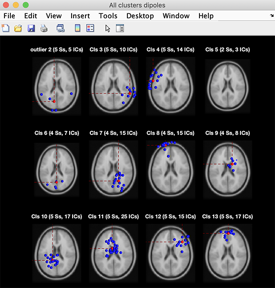
Selecting one of the clusters from the list shown in the upper left box displays a list of the cluster components in the text box on the upper right. The All cluster centroids option in the (left) text box list will cause the function to display results for all but the ParentCluster. Selecting one of the plotting options will then show all cluster centroids in a single figure. To review all cluster dipole locations, press the Plot dipoles button in the left column. This will open the plot viewer showing all the cluster component dipoles (in blue), plus the cluster mean dipole location (in red). Not surprisingly, components have been clustered in groups of dipoles with distinct locations.
You may also review cluster scalp maps, by pressing the Plot scalp maps option. This will produce the figure below:
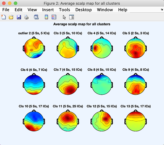
Note that your exact clusters might differ slightly since the kmean algorithm starts from a random assignment of components to clusters.
In computing the mean cluster scalp maps (or scalp map centroids), the polarity of each of the cluster’s component maps was first adjusted so as to correlate positively with the cluster mean (recall that component maps have no absolute polarity). Then the map variances were equated. Finally, the normalized means were computed.
To see individual component scalp maps for components in the cluster, select the cluster of interest in the left column (for example, Cluster 6 as in the figure above). Then press the Plot scalp maps option in the right column. The following figure will appear (Note that, in your case, this cluster might be a different index).
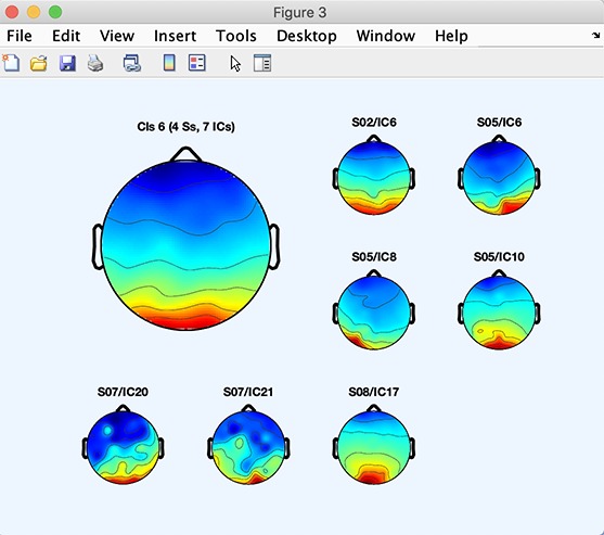
Here, SO2 IC6 means independent component 6 for subject SO2, etc.
Note that channels missing from any of the datasets do not affect clustering or visualization of cluster scalp maps. Component scalp maps are interpolated by the toporeplot.m function, avoiding the need to restrict STUDY datasets to a common always clean channel subset or to perform missing channel interpolation on individual datasets.
You may also plot scalp maps for individual components in the cluster by selecting components in the right column and then pressing Plot scalp maps (not shown).
You may plot the dipoles for this cluster. Press the Plot dipoles button in the left or right column. The following image pops up.
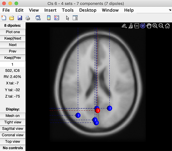
Scroll through the dipoles one by one, rotating the plot in 3-D or selecting among the three cardinal views (lower left buttons), etc. Information about the plotted dipoles is presented in the left-center side bar (see the image above).
Let’s also plot the spectrum for this cluster along with the spectrum of the individual components. In the right column, click on the Plot spectra button.
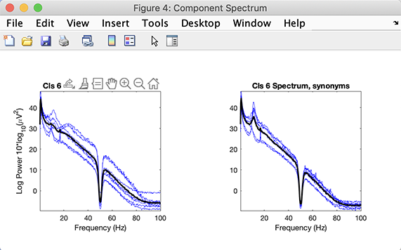
We can see a clear 10 Hz peak in all the components of this cluster. Let’s finally plot the ERPs for the two conditions of this STUDY. Click on the Params button in the central column adjacent to the Plot ERPs buttons. Change the time range to -200 ms to 1000 ms as shown below. Check the checkbox to plot the first independent variable on the same plot. Press Ok.
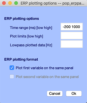
Then click on the Plot ERPs button in the right column. The following window pops up.
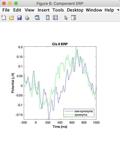
Here Cluster 6 accounts for some central occipital alpha activity – note the strong 10-Hz peak in the activity spectra. The cluster ERPs show a very slow (1-Hz) pattern. The apparent latency shift between conditions in the slow wave activity may or may not be significant.
To quickly recognize the nature of component clusters by their activity features requires experience (see the ICA decomposition tutorial for more information).
Editing clusters
The results of clustering can also be updated manually in the cluster viewing and editing window (called from the Study → Edit/plot clusters menu item). These editing options allow flexibility for adjusting the clustering results. Components can be reassigned to different clusters, new clusters can be created, and outlier components can be rejected from a cluster. Note that if you make changes via the pop_clustedit.m GUI, then wish to cancel these changes, pressing the Cancel button will cause the STUDY changes to be forgotten.

We describe below the four button to edit clusters.
-
Renaming a cluster. The Rename selected cluster option allows you to rename any cluster using a (mnemonic) name of your choice. Pressing this option button opens a pop-up window asking for the new name of the selected cluster. For instance, if you think a cluster contains components accounting for eye blinks you may rename it “Blinks”.
-
Removing selected outlier components manually. You may remove outlier components from a cluster manually. This option allows you to de-select seeming outlier components irrespective of their distance from the cluster mean. To manually reject components, first select the cluster of interest from the list on the left, then select the desired outlier component(s) from the component list on the right, then press the Remove selected outlier comps button. A confirmation window will pop up.
-
Creating a new cluster. To create a new empty cluster, press the Create new cluster option. This opens a pop-up window asking for a name for the new cluster. If no name is given, the default name is ‘Cls #’, where ‘#’ is the next available cluster number. For changes to take place, press the Ok button in the pop-up window. The new empty cluster will appear as one of the clusters in the list on the left of the editing/viewing cluster window.
-
Reassigning components to clusters. To move components between any two clusters, first select the origin cluster from the list on the left, then select the components of interest from the component list on the right, and press the Reassign selected component(s) option button. Select the target cluster from the list of available clusters.
Further component clustering consideration
Multiple components from the same subjects in ICA clusters
When plotting ICA clusters, EEGLAB allows by default several components from the same subject to be included in a given cluster. This can sometimes cause problems when using statistics.
When you include more than one component from the same subject, you are not making inferences about the general population of subjects anymore but instead about components of the specific subjects you are studying. It is all a matter of how many components you have per subject compared to the number of subjects.
For example, if you have on average one component per subject (some subjects having 0, some other two components in the cluster), and you have 200 subjects, then the original null hypothesis (which allows making inferences about the general population of subjects) is mostly preserved. If you have 10 subjects and 10 components of the same subject in a given cluster, it is not.
In general, when multiple components from the same subjects in ICA clusters becomes a problem, we prefer to use at most one component per subject per cluster because this avoids having to compromise with the statistics (this is possible when using the EEGLAB Corrmap plugin for clustering data). Alternatively, remove components manually in clusters.
Choice of STUDY design for clustering
When preclustering ICA components, the current STUDY design is taken into account.
For example, if you have two conditions per subject and both conditions share the same set of ICA components, then during preclustering, when computing the component distance measure used for clustering, data measures from both conditions are concatenated. For example, when using the mean power spectrum to cluster components, instead of having say 50 spectral values (one per frequency) for each component, during preclustering 100 values (two sets of 50 frequencies, one for each condition) will be placed one after the other. EEGLAB will not allow you to cluster components using a STUDY design that does not include all STUDY datasets. Note that you are using anatomical component information only (scalp topographies and/or equivalent dipoles) and no other measures to cluster components, then the STUDY design does not impact the clustering solution.
To precluster, therefore, we advise using the simplest STUDY design possible. Often, this is the one that is most natural for the experiment. After clustering, since all ICA components are included in the clustering, ICA clusters are constant for all conditions and STUDY designs. Thus, once your components are clustered, it is possible to compare cluster activities for any STUDY design.
Comparing clusters’ activity in different conditions
Once ICA components are clustered, it is possible to compute differences between conditions using any STUDY design. Whenever you select a different design, ICA components are assigned to the conditions in the design according to your design as per the clustering solution. For example, if you have only one ICA decomposition per subject and a 2x1 design (2 conditions, 1 subject group, collected in 1 session), then both conditions share the same components.
Comparing activities of ICA components between conditions is like comparing activities in different data channels. Comparing the activities of a cluster of components between conditions could be seen as similar to comparing the activity of a given channel across subjects. Remember that ICA components and electrode channels are both spatial filters. Each data channel is the arithmetic difference between the potential reaching some scalp electrode and the potential reaching a reference electrode (or the mean of the potentials reaching the set of reference electrodes). Each ICA component gives the arithmetic weighted sum/difference of the signals reaching each of the electrodes. Here the negatively weighted electrode signals can be said to serve the role of the reference channel (although this channel combination will typically be different for each component).
For STUDY designs in which component activities of two subject groups are to be compared, the computed measure differences will be between components for each group within each cluster.
Try it on your own data
Note that with only a few subjects and a few clusters (a necessary limitation to distribute the tutorial example easily), it may not be possible to find consistent component clusters with uniform and easily identifiable natures. We have obtained much more satisfactory results when clustering data from 15 to 30 or more subjects.
After following this tutorial using the sample data, we recommend you create a study for a larger group of datasets whose properties you know well. Then try clustering components of this study in several ways. Carefully study the consistency and properties of the generated component clusters to determine which method of clustering produces clusters adequate for your research purposes.