This section provides a demonstration of the use of SIFT to estimate and visualize source-domain information flow dynamics in an EEG dataset. To get the most of this tutorial you may want to download the toolbox and sample data and follow along with the step-by-step instructions. The toolbox is demonstrated through hands-on examples primarily using SIFT’s Graphical User Interface (GUI). Theory boxes provide additional information and suggestions at some stages of the SIFT pipeline.
In order to make the most use of SIFT’s functionality, it is important to first separate your data into sources – e.g. using EEGLAB’s built-in Independent Component Analysis (ICA) routines. To make use of the advanced network visualization tools, these sources should also be localized in 3D space e.g. using dipole fitting (pop_dipfit()). Detailed information on performing an ICA decomposition and source localization can be found in the EEGLAB wiki. In this example we will be using two datasets from a single subject performing a two-back with feedback continuous performance task depicted in the figure below (Onton and Makeig, 2007). Here the subject is presented with a continuous stream of letters, separated by ~1500 ms, and instructed to press a button with the right thumb if the current letter matches the one presented twice earlier in the sequence and press with the left thumb if the letter is not a match. Correct and erroneous responses are followed by an auditory “beep” or “boop” sound. Data is collected using a 64-channel Biosemi system with a sampling rate of 256 Hz. The data is common-average re-referenced and zero-phase high-pass filtered at 0.1 Hz. The datasets we are analyzing are segregated into correct (RespCorr) and incorrect (RespWrong) responses, time-locked to the button press and separated into maximally independent components using Infomax ICA (Bell and Sejnowski, 1995). These sources are localized using a single or dual-symmetric equivalent-current dipole model using a four-shell spherical head model co-registered to the subjects’ electrode locations by warping the electrode locations to the model head sphere using tools from the EEGLAB dipfit plug-in.
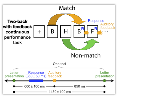
Figure caption. Two-back with feedback CPT (Onton and Makeig, 2007).
In this exercise, we will be analyzing the information flow between several of these anatomically localized sources of brain activity during correct responses and error commission.
The SIFT sub-menu options correspond to SIFT’s five main modules: Pre-Processing, Model Fitting and Validation, Connectivity Analysis, Statistics, and Visualization.
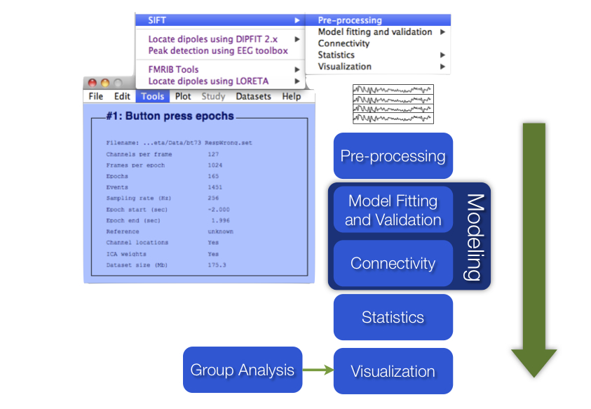
Figure caption. SIFT Data processing pipeline