Time/frequency decomposition
Time/frequency analysis characterizes changes or perturbations in the spectral content of the data considered as a sum of windowed sinusoidal functions (i.e., sinusoidal wavelets). There are a long history and much recent development of methods for time/frequency decomposition. The methods used in the basic EEGLAB functions are straightforward. Their mathematical details are given in a reference paper (Delorme and Makeig, 2004). You may also want to watch the short series of videos on computing time-frequency decompositions in EEGLAB (hosted on Youtube) below. If you click on the icon on the top right corner, you can see the list of all the videos in the playlist.
ERSP and ITC time-frequency analysis
Time-frequency images
We use here the tutorial dataset as it was after extracting data epochs. Select the File → load existing dataset menu item and select the tutorial file “eeglab_data_epochs_ica.set” located in the “sample_data” folder of EEGLAB. Then press Open.
To detect transient event-related spectral perturbation, or ERSP, (Makeig, 1993) (event-related shifts in the power spectrum) and inter-trial coherence (ITC) (event-related phase-locking) events in epoched EEGLAB datasets, select Plot → Time-frequency transforms → Channel time-frequency calling the pop_newtimef.m function. Below, we enter 14 (Cz) for the Channel number. We let the other defaults remain. We press Ok.
Note the default “Wavelet cycles” entry is 3 0.8. As explained in the help message for the newtimef.m function, this means that the wavelet used to measure the amount and phase of the data in each successive, overlapping time window will begin with a 3-cycle wavelet (with a Hanning-tapered window applied). The ‘0.8’ here means that the number of cycles in the wavelets used for higher frequencies will continue to expand slowly, reaching 20% (1 minus 0.8) of the number of cycles in the equivalent FFT window at its highest frequency. This controls the shapes of the individual time/frequency windows measured by the function and their shapes in the resulting time/frequency panes.
Note: This information does not set the lowest frequency to be analyzed. By current default, the lowest frequency window is about 0.5 seconds long. Using three cycles in 0.5 seconds sets the lowest frequency analyzed to about 6 Hz. To make this lowest frequency near 3 Hz, we would need to add the optional newtimef.m argument “ ‘winlen’, xxx “ where xxx is the sampling rate of the data (also shown on the blue EEGLAB menu window). This would specify that the window length (‘winlen’) at the lowest frequency should be xxx samples long (i.e., 1 sec long). If we were using 1 cycle, the lowest frequency would be 1 Hz. With 3 cycles, the lowest frequency is 3 Hz.
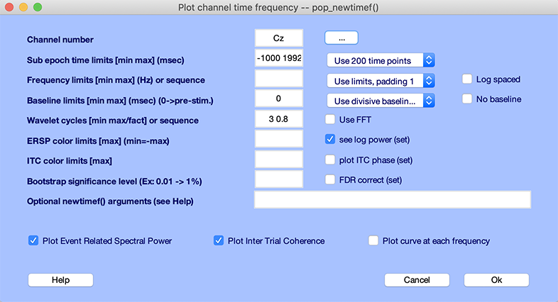
The window below appears:
-
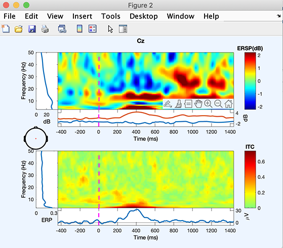
The top image shows mean event-related changes in spectral power (from pre-stimulus baseline) at each time during the epoch and at each frequency (< 50 Hz). To inspect these changes more closely, click on the color image. A new window will pop up. Enabling MATLAB zoom allows zooming into any desired time/frequency window. The ERSP image shows a brief decrease in power at about 370 ms at 8 Hz (click on the image to zoom in and determine the exact frequency), a power increase centered at 13.5 Hz and starting at 300 ms. More spectral changes occur at 20-28 Hz. The left panel adjacent to the top image shows the baseline mean power spectrum, and the lower part of the top image, the ERSP envelope (low and high mean dB values, relative to baseline, at each time in the epoch).
-
The lower image shows the Inter-Trial coherence (ITC) at all frequencies. We previously encountered the ITC when we explained the ERP image plotting. A significant ITC indicates that the EEG activity at a given time and frequency in single trials becomes phase-locked (not phase-random with respect to the time-locking experimental event). Here, ITC briefly increases at about 10 Hz (at about the same time as the power increase in the upper panel).
The help message for the newtimef.m function contains information about its parameters, the images and curve plotted, and their meanings.
Note: You may change the optional parameter padratio to increase frequency resolution. For example, setting the padratio to 16 would give a smooth looking plot at quite some unnecessary computational cost.
Masking for significance
Select Plot → Channel time-frequency and enter 14 (Cz) for the Channel number. Use .05 for the Bootstrap significance level, and check the FDR correct checkbox to correct for multiple comparisons using the False Discovery Rate method (see statistics Appendix for more information). Press Ok.
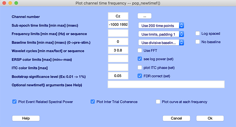
The window below appears:
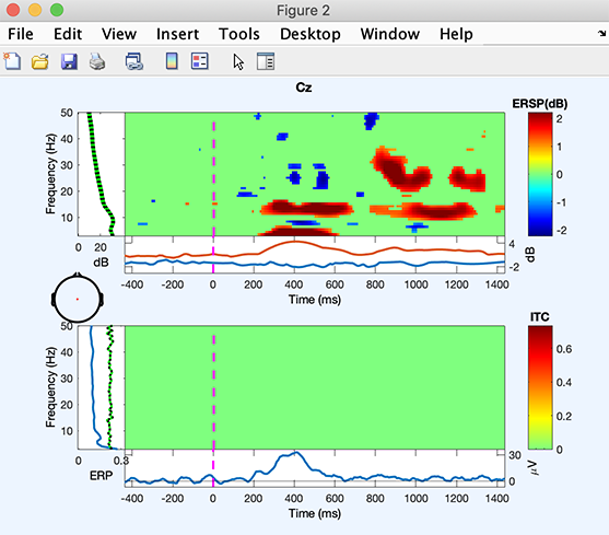
Note that the time/frequency points showing significant ITC and ERSP are not necessarily identical. ERSP reaches significance over the regions described in the previous section. However, ITC does not reach significance. Note also that the method used to assess significance is based on random data shuffling, so these features’ exact significance limits may appear slightly different.
Time-frequency curves
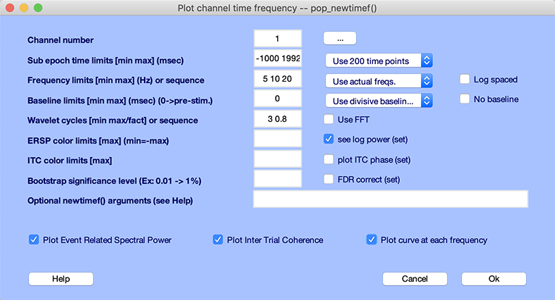
In addition to plotting time-frequency images, it is also possible to plot time-frequency curves at given frequencies. Select Plot → Channel time-frequency and enter
- 1 (FPz) for the Channel number
- Enter 5 10 20 in the Frequency limit edit box and select Use actual freq. in the adjacent dropdown list
- Check the checkbox Plot curve at each frequency
Press Ok.
The window below appears:
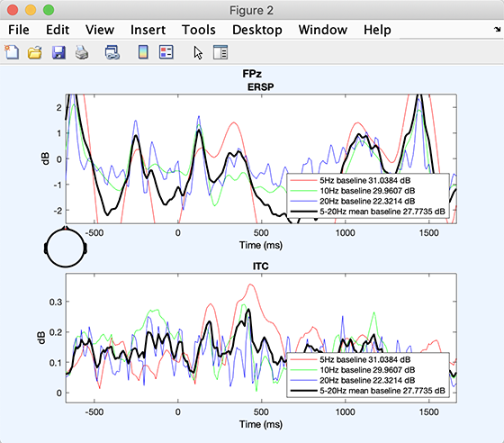
The plot above shows fluctuations in spectral power and ITC through time at the chosen frequencies. This plotting format does not allow masking for significance.
Advanced ERSP/ITC plotting
Recall that spectral perturbations at a single-analysis frequency and channel in the single epochs (sorted by some relevant value) can be imaged using erpimage.m or by selecting menu item Plot → Component → Channel ERP image.
Called from the command line, the pop_newtimef.m and newtimef.m routines can return the data for each part of their figures as a MATLAB variable. Accumulating the ERSP and ITC images (plus the ERSP baseline and significance-level information) for all channels allows using another toolbox routine, tftopo.m (currently unavailable from the EEGLAB menu). See the EEGLAB script writing tutorial for more details.