Equivalent dipole source localization of EEG or ERP data
Table of contents
Using DIPFIT to fit one dipole to EEG or ERP scalp maps
EEGLAB provides a command-line implementation of the DIPFIT plugin to fit dipoles to raw ERP or EEG scalp maps that has otherwise not been expressly designed anywhere else. Fitting may only be performed at selected time points, not throughout a time window. First, you must specify the DIPFIT settings on the selected dataset. Then, to fit a time point at 100 ms in an average ERP waveform (for example) from the main tutorial data set, use the following MATLAB commands.
eeglab; close; % add path
eeglabp = fileparts(which('eeglab.m'));
EEG = pop_loadset(fullfile(eeglabp, 'sample_data', 'eeglab_data_epochs_ica.set'));
% Find the 100-ms latency data frame
latency = 0.100;
pt100 = round((latency-EEG.xmin)*EEG.srate);
% Find the best-fitting dipole for the ERP scalp map at this timepoint
erp = mean(EEG.data(:,:,:), 3);
dipfitdefs;
% Use MNI BEM model
EEG = pop_dipfit_settings( EEG, 'hdmfile',template_models(2).hdmfile,'coordformat',template_models(2).coordformat,...
'mrifile',template_models(2).mrifile,'chanfile',template_models(2).chanfile,...
'coord_transform',[0.83215 -15.6287 2.4114 0.081214 0.00093739 -1.5732 1.1742 1.0601 1.1485] ,'chansel',[1:32] );
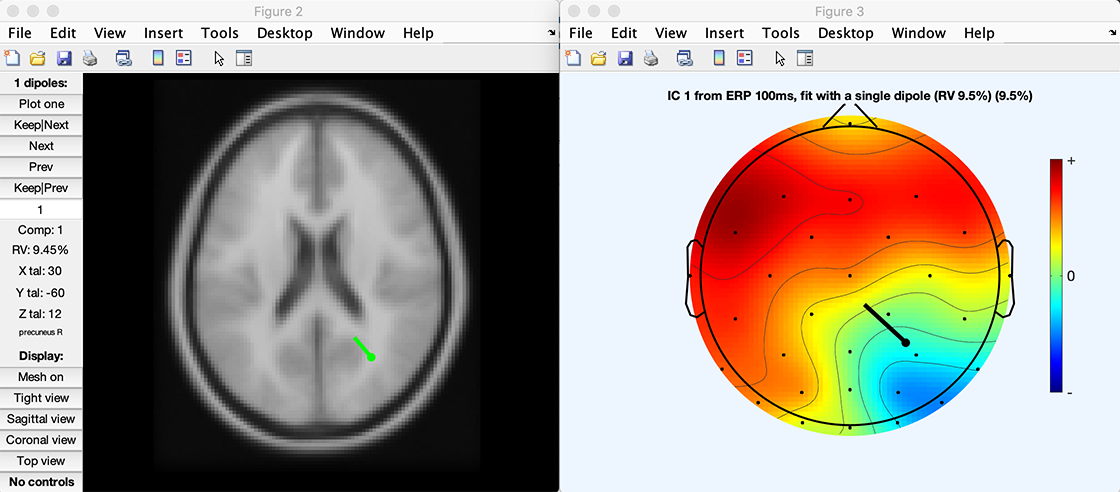
[ dipole, model, TMPEEG] = dipfit_erpeeg(erp(:,pt100), EEG.chanlocs, 'settings', EEG.dipfit, 'threshold', 100);
% plot the dipole in 3-D
pop_dipplot(TMPEEG, 1, 'normlen', 'on');
% Plot the dipole plus the scalp map
figure; pop_topoplot(TMPEEG,0,1, [ 'ERP 100ms, fit with a single dipole (RV ' num2str(dipole(1).rv*100,2) '%)'], 0, 1);
Click here to download the script above. When running the script, the two plots below are created.
It is also possible to locate EEG/ERP sources using eLoreta. We have written a simple plugin for that purpose. This plugin was designed in a minimalist fashion so it could be used as a template for other similar plugins. Its graphical output is the same as the script shown in the next section.
Advanced source reconstruction using DIPFIT/FieldTrip
Background: DIPFIT relies on FieldTrip, though in fact, DIPFIT was also an ancestor of FieldTrip: when Robert Oostenveld, the first FieldTrip developer, decided to release source imaging functions he had developed during his dissertation work, he first packaged them in EEGLAB as DIPFIT. A few years later, when he and his collaborators released FieldTrip (also running on MATLAB), we reworked DIPFIT so it would use the FieldTrip functions that Robert and colleagues planned to and have since maintained for use in FieldTrip. Below is a short tutorial on how to perform source modeling using FieldTrip applied to data in an EEGLAB dataset.
Implementation: First, use DIPFIT to align the electrode locations with a head model of choice (menu item Tools → Locate dipoles using DIPFIT → Head model and settings). The resulting DIPFIT information may then be used to perform source localization in FieldTrip.
Performing source reconstruction in a volume
The first snippet of code below creates the leadfield matrix for a 3-D grid (for example, for use with eLoreta).
%% First load a dataset in EEGLAB.
% Then use EEGLAB menu item <em>Tools > Locate dipoles using DIPFIT > Head model and settings</em>
% to align electrode locations to a head model of choice
% The eeglab/fieldtrip code is shown below:

eeglab                        % start eeglab
eeglabPath = fileparts(which('eeglab'));                 % save its location
bemPath = fullfile(eeglabPath, 'plugins', 'dipfit', 'standard_BEM');    % load the dipfit plugin
EEG = pop_loadset(fullfile(eeglabPath, 'sample_data', 'eeglab_data_epochs_ica.set'));   % load the sample eeglab epoched dataset
EEG = pop_dipfit_settings( EEG, 'hdmfile',fullfile(bemPath, 'standard_vol.mat'), ...
           'coordformat','MNI','mrifile',fullfile(bemPath, 'standard_mri.mat'), ...
           'chanfile',fullfile(bemPath, 'elec', 'standard_1005.elc'), ...
           'coord_transform',[0.83215 -15.6287 2.4114 0.081214 0.00093739 -1.5732 1.1742 1.0601 1.1485] , ...
           'chansel',[1:32] );
Then calculate a volumetric leadfield matrix using FieldTrip function ft_prepare_leadfield. Note that the head model is also used to assess whether a given voxel is within or outside the brain.
%% Leadfield Matrix calculation
dataPre = eeglab2fieldtrip(EEG, 'preprocessing', 'dipfit');   % convert the EEG data structure to fieldtrip

cfg = [];
cfg.channel = {'all', '-EOG1'};
cfg.reref = 'yes';
cfg.refchannel = {'all', '-EOG1'};
dataPre = ft_preprocessing(cfg, dataPre);

vol = load('-mat', EEG.dipfit.hdmfile);

cfg            = [];
cfg.elec       = dataPre.elec;
cfg.headmodel  = vol.vol;
cfg.resolution = 10;   % use a 3-D grid with a 1 cm resolution
cfg.unit       = 'mm';
cfg.channel    = { 'all' };
[sourcemodel] = ft_prepare_leadfield(cfg);
Then use the now generated leadfield matrix to perform source reconstruction. Below, we provide a simple example, to model putative sources of ERP features using eLoreta. Here, eLoreta may be replaced by other approaches, such as Dynamical Imaging of Coherent Sources ‘dics’ (see the FieldTrip tutorial page from which this section is inspired for more information).
%% Compute an ERP in FieldTrip. Note that the covariance matrix needs to be calculated here for use in source estimation.
cfg                  = [];
cfg.covariance       = 'yes';
cfg.covariancewindow = [EEG.xmin 0]; % calculate the average of the covariance matrices
                                   % for each trial (but using the pre-event baseline  data only)
dataAvg = ft_timelockanalysis(cfg, dataPre);

% source reconstruction
cfg             = [];
cfg.method      = 'eloreta';
cfg.sourcemodel = sourcemodel;
cfg.headmodel   = vol.vol;
source          = ft_sourceanalysis(cfg, dataAvg);  % compute the source model
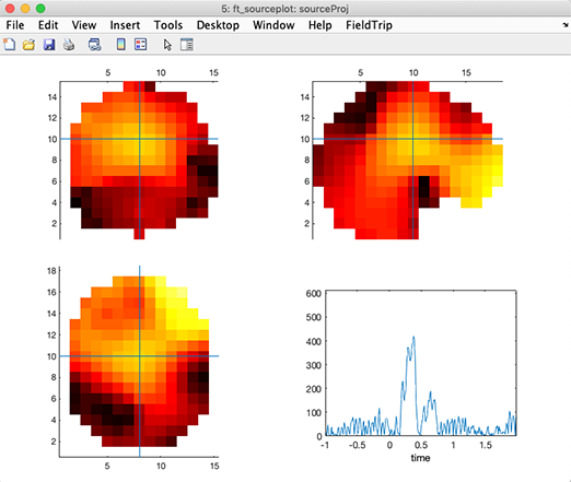
Then plot the solution using FieldTrip functions. Note that the solutions are generated in a low-resolution head volume. It is not technically feasible to interpolate this volume onto a high-resolution MRI in (near) real-time – online, it would require too many computational resources, while offline, it would require too much memory (one head volume at every latency. Unlike fMRI data, EEG data have a high temporal resolution, so the low-resolution head volume x latencies matrix is already quite large - transforming it into a high-resolution volume matrix is impractical). Note that you will need to click on different voxels and latencies to obtain a figure that looks like the one below.
Note also that you can see discontinuities in the plotted volume. This is because of sudden inversion of the polarity of the dipole orientation in the nearest voxels. This is normal. The product of voxel polarity by temporal activity remains continuous in space and time. Still, because of the projection method for the 3-D dipole orientation at the voxel level, neighboring voxels may have opposite polarities (and, of course, oppositely-signed time courses as well). An ideal solution has not been found yet to avoid inversions in both space and time - having all dipoles point outwards with respect to the head center - and inverting associated source time courses accordingly - would be a solution worth trying. Or we could plot the different axes of dipole orientation.
%% Plot Loreta solution
cfg = [];
cfg.projectmom = 'yes';
cfg.flipori = 'yes';
sourceProj = ft_sourcedescriptives(cfg, source);

cfg = [];
cfg.parameter = 'mom';
cfg.operation = 'abs';
sourceProj = ft_math(cfg, sourceProj);

cfg              = [];
cfg.method       = 'ortho';
cfg.funparameter = 'mom';
figure; ft_sourceplot(cfg, sourceProj);
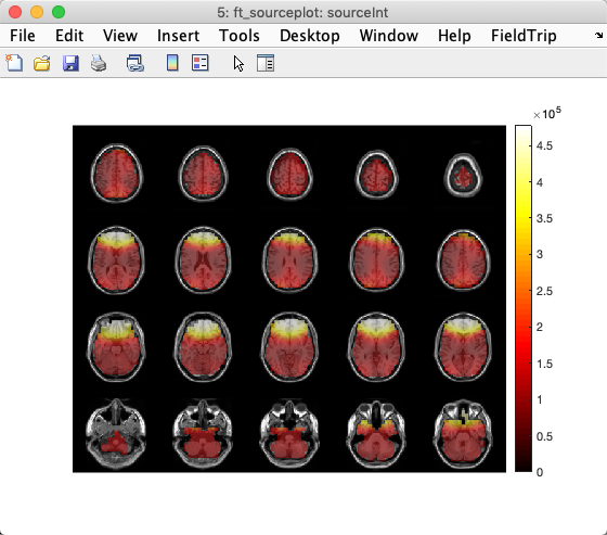
Once latencies of interest have been chosen, they may be projected into a high-resolution MRI. head image. Below, we show global power on MRI slices of a template brain.
%% project sources on MRI and plot solution
mri = load('-mat', EEG.dipfit.mrifile);
mri = ft_volumereslice([], mri.mri);

cfg              = [];
cfg.downsample   = 2;
cfg.parameter    = 'pow';
source.oridimord = 'pos';
source.momdimord = 'pos';
sourceInt  = ft_sourceinterpolate(cfg, source , mri);

cfg              = [];
cfg.method       = 'slice';
cfg.funparameter = 'pow';
ft_sourceplot(cfg, sourceInt);
Performing source reconstruction on a surface
Alternatively, the code below generates a leadfield matrix for a realistic 3-D mesh in MNI space. Note that this requires that you choose the MNI BEM head model when selecting the head model in the DIPFIT settings menu. Different mesh versions are available using different resolutions. Refer to this FieldTrip tutorial for more information. Note that the code below assumes that you have run the code above.
%% Prepare leadfield surface
[ftVer, ftPath] = ft_version;
sourcemodel = ft_read_headshape(fullfile(ftPath, 'template', 'sourcemodel', 'cortex_8196.surf.gii'));

cfg           = [];
cfg.grid      = sourcemodel;    % source points
cfg.headmodel = vol.vol;        % volume conduction model
leadfield = ft_prepare_leadfield(cfg, dataAvg);
The code in the previous section used eLoreta. In this section we will use minimal norm estimate (MNE). Both MNE and eLoreta can perform source reconstruction at each latency (assuming you are using an EEG time series as input).
%% Surface source analysis
cfg               = [];
cfg.method        = 'mne';
cfg.grid          = leadfield;
cfg.headmodel     = vol.vol;
cfg.mne.lambda    = 3;
cfg.mne.scalesourcecov = 'yes';
source            = ft_sourceanalysis(cfg, dataAvg);
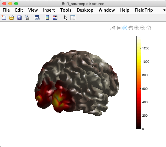
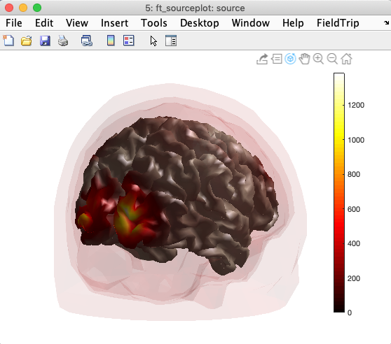
Now we will plot global power. Using the same approach, it is possible to create movies in which the MNE source solutions evolves over time, as described on this page.
%% Surface source plot
cfg = [];
cfg.funparameter = 'pow';
cfg.maskparameter = 'pow';
cfg.method = 'surface';
cfg.latency = 0.4;
cfg.opacitylim = [0 200];
ft_sourceplot(cfg, source);
You may also visually check the alignment of the source model mesh with the BEM head model mesh by overlaying the BEM mesh on the image above, as shown below
hold on; ft_plot_mesh(vol.vol.bnd(3), 'facecolor', 'red', 'facealpha', 0.05, 'edgecolor', 'none');
hold on; ft_plot_mesh(vol.vol.bnd(2), 'facecolor', 'red', 'facealpha', 0.05, 'edgecolor', 'none');
hold on; ft_plot_mesh(vol.vol.bnd(1), 'facecolor', 'red', 'facealpha', 0.05, 'edgecolor', 'none');
Click here to download the script above.
Relevant FieldTrip tutorials
- How to build a source model and available template source models (one of them is used above)
- How to define the volume conduction model
- Beamformer methods - note that you may replace ‘dics’ by ‘eloreta’ in this tutorial
- Minimum norm estimates for MEG, but can be adapted for EEG
- Previous tutorial version of DIPFIT
This section was written by Arnaud Delorme with contributions and feedback from Robert Oostenveld and Scott Makeig.