EEGLAB Filtering FAQ

Q. What are passband, stopband, transition bandwidth, cutoff frequency, passband ripple/ringing, and stopband ripple/attenuation?

A. You can find explanations in this PDF presentation created by Andreas Widmann.

Q. What is the difference between the “Basic FIR filter (legacy)” and the “Basic FIR filter (new)”? Which should I use?

A. The heuristic for automatically determining the filter length in the legacy basic FIR filter (pop_eegfilt) was inappropriate (possibly causing suboptimal filtering or unexpected filter effects). The new basic FIR filter (pop_eegfiltnew) has a new heuristic for automatically determining the filter length and is based on the Firfilt plugin. The legacy function should only be used for backward compatibility purposes.

Q. What is the difference between the “Basic FIR filter (new)” and the “Windowed sinc FIR filter”?

A. Both are based on windowed sinc filters. The basic filter applies a hardcoded hamming window, has an automatic default for filter length, and is defined by the passband edges. The windowed sinc FIR filter allows manual selection of window type, estimation of filter length by transition bandwidth (no default), and is defined by cutoff frequencies (-6dB, half amplitude).

Q. Why does Firfilt-plugin run faster than the legacy EEGLAB filter?

A. The Firfilt plugin does not use filtfilt to achieve zero-phase but shifts the signal by the filter’s group delay (NB: requiring ODD filter length/even filter order). So, the data are only filtered once with multi-threading (filtfilt does not seem to be multi-threading capable).

Q. What is the recommended passband ripple/stopband attenuation/window type?

A. Ripple, i.e. deviation from the requested frequency response (0 in stopband, 1 in passband) is equal in passband and stopband in windowed sinc FIR filters. Ripple/attenuation is defined by the window type. 0.002 to 0.001 (that is, 0.2 to 0.1%; Hamming or Kaiser window) are reasonable starting values. This equals a stopband attenuation of -53 to -60 dB which is ok.

Q. Should we prefer separate high- and low-pass filters over bandpass filters? (09/30/2020 updated)

A. With separate high- and low-pass filters, transition bandwidth can be defined independently. High-pass filters often require narrower transition bands than low-pass filters. Separate filtering is preferable in these cases.

Q. What is the difference between filter length and filter order?

A. Filter order is defined as filter length minus 1.

Q. What is the transition band?

A. The transition band is the frequency band/range between the passband edge and the stopband edge. In windowed sinc FIR filters the -6dB cutoff is in the center of the transition band.

Q. What is the slope of windowed sinc FIR filters in dB/oct (as in IIR filters)?

A. Slope CANNOT be defined in dB/oct for windowed sinc FIR filters. Rather use transition bandwidth. There is no straightforward conversion of slope in dB/oct to transition bandwidth due to conceptual differences between FIR and IIR filters. IIR filters do not have a defined stopband.

Q. What is the lower limit for cutoff frequency for high-pass filter?

A. There is no theoretical lower limit, however, the lower the cutoff the steeper is the roll-off and the higher is the filter order (length). Very low cutoff frequencies as low as 0.01 Hz as sometimes found in the literature require extremely long filters (FIR) or are prone to instability (IIR). The computation time for very long FIR filters becomes enormous. You can try the ‘usefftfilt’ option in “Basic FIR Filter (new, default)” (pop_eegfiltnew) or “Windowed sinc FIR Filter” (pop_firws) to speed up filtering for FIR filter orders higher than 2000 to 3000. Note that lowering the sampling rate also reduces the required filter orders. If you are experiencing stability problems with IIR filters with lower cutoff frequencies, also consider reducing the sampling frequency of the signal.

Q. What is the recommended transition bandwidth (for a windowed sinc FIR high-pass filter)?

A. Generally, the slope in the frequency domain should be as low/flat as possible, that is the transition band as wide as possible. Steeper slopes reduce the precision in the time domain; distortions and artifacts are additionally spread wider due to the longer filter length. A good staring value for a high-pass filter: twice the cutoff frequency (-6 dB) for cutoff <= 1 Hz, 2 Hz for cutoff frequency < 1 and <= 8 Hz and 25% of cutoff frequency for cutoff > 8 Hz. This is also the heuristic implemented in the new basic FIR filter (generalized for all critical frequencies). However, please note, that it is recommended to (manually) adjust this heuristic to the application of interest. Do not go beyond twice of the cutoff frequency (i.e., transition band goes below DC/0 Hz). TIP: Strong attenuation (<< -60dB) can be important for DC/0 Hz (e,g,, to get rid of the DC offset for Biosemi files or to avoid baseline correction). By using twice of the cutoff frequency for transition bandwidth, a type 1 windowed sinc filter can be tuned for excellent DC attenuation.

Q. What stopband attenuation is good?

A. The community default of Hamming window/-53dB is a good starting value. With Kaiser windows stopband attenuation can be precisely adjusted.

Q. How can I find optimal values for cutoff frequencies, attenuation, and filter length for my particular application?

A. By testing and systematically comparing the effects of different filters on the signal in the time domain.

Q. Where can I read more about windowed sinc FIR filters?

A. Check out Engineers guide to digital signal processing.

Q. For Granger Causality analysis, what filter should be used? (11/21/2020 Updated)

A. There are a few important things to confirm.

• Barnett and Seth (2011) showed that multivariate Granger causality is in theory invariant under zero-phase (a.k.a. phase-invariant) filter. They do recommend filtering to achieve stationarity (e.g., drift, line noise) See Seth, Barrett, Bernett (2015).
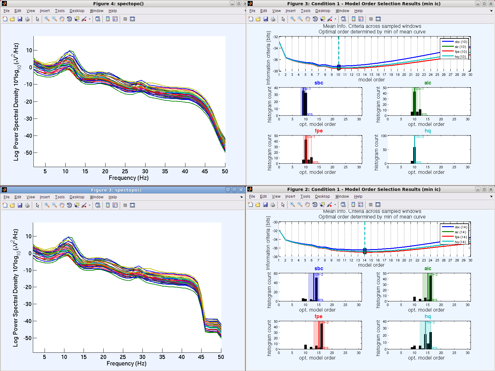
• However, in practice, filtering causes problems in calculating multivariate Granger causality. The main problem is the increase in model order. This is because filtering makes the power spectrum density of the signal complicated (low power in the stopband, steep roll-off, etc). See the following example: 33ch EEG, downsampled to 100 Hz, without (top) and with (bottom) applying 44.5Hz low-pass filter (FIR, Blackman, TBW 1 Hz). Notice that the estimated model orders is worsened from 10 (without LPF) to 14 (with LPF)–but apparently taking 16 (with LPF) is the right decision here from AIC, FPE and HQ results.

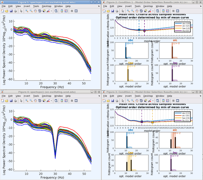
Here is another comparison: with and without notch filter at 30Hz (cutoff freq 28 and 32Hz, TBW 0.5Hz). Note the suggested order became 10-12 to 11-15 with the notch filter on.

• The second problem, which comes from the same reason mentioned above, is that empirical estimates of VAR parameters yields unstable models due to poor parameter estimate for increased model order.
• The third problem is that filtering causes numerical instabilities in estimating causality.

How can we address these problems?

• When applying a high-pass filter to achieve stationarity, let the transition band end at DC (i.e. 0Hz). For example, when you use EEGLAB’s ‘Basic FIR filter (new, default)‘ to apply high-pass filter with ‘passband edge’ below 2-Hz, the transition band is automatically adjusted so that it always ends at DC. (We use 1-Hz high-pass for the ICA purpose; empirical test is required to see whether 2-Hz high-pass is beneficial for GCA compared with 1-Hz). If you want to set the high-pass filter passband edge above 2 Hz, we recommend you use ‘Windowed sinc FIR filter’ to design the filter so that it has the stopband at DC. (CAUTION: ‘Windowed sinc FIR filter’ uses cutoff frequency and not passband edge i.e. cutoff frequency of 1 Hz is equivalent to passband edge at 2 Hz
• When treating the line noise, use CleanLine() instead of notch filter because the former is phase-invariant.
• When downsampling data (which is useful for multivariate Granger causality analysis), use mild anti-aliasing filter and do not let the stopband below the Nyquist frequency. In practice, use the following example. In this example, you are downsampling your data to 200Hz (i.e., Nyquist frequency is 100Hz), with the cutoff frequency being 80Hz (i.e. 100Hz*0.8) and the transition bandwidth 40Hz (i.e. 100Hz*0.4).

  EEG = pop_resample(EEG, 200, 0.8, 0.4);
  

Q. When should causal filters be used? (3/15/2021)

Causal filters typically should only be used if the application explicitly requires this. For example, if causality matters as in the detection of onset latencies (even if the problem is overestimated as it mainly affects ultra-sharp transients typically not observed in EEG/ERP), the analysis of small fast components before large slow components (e.g. if higher high-pass cutoff frequencies are required), or in the analysis of pre-stimulus activity, that is, your case. The difference between a linear causal and linear non-causal filter is exclusively the time axis. The output of the non-causal filter equals the delay corrected output of the causal filter. It is sufficient to change the EEG.times time axis. That is, if your signal of interest is further away from stimulus onset than the group delay, you can simply use a linear non-causal filter.

% Example:

    sig = [ 0 0 0 0 0 1 0 0 0 0 0 ]; % test signal (impulse)
    b = [ 1 1 1 1 1 ] / 5; % some crude boxcar filter for demonstration purposes only, linear-phase, length = 5, order = 4, group delay = 2
    fsig = filter( b, 1, sig ); % causal filter
    plot( -5:5, [ sig; fsig ]', 'o' ) % the filtered impulse in the output does not start before the impulse in the input
    fsig = filter( b, 1, [ sig 0 0 ] ) % padded causal filter
    fsig = fsig( 3:end ); % delay correction by group delay, this is what makes the filter non-causal and zero-phase
    plot( -5:5, [ sig; fsig ]', 'o' ) % the filtered impulse in the output starts before the impulse in the input BUT everything before x = -2 is unaffected

Q. Should I use a linear causal FIR filter with delay correction or a non-linear causal filter (e.g. minimum-phase)?

You cannot delay correct a causal filter (linear or non-linear). This would make it automatically non-causal and break causality and there is no way around this. If the (group) delay is too large for your purpose, you must reduce the delay and thus use a non-linear filter (e.g. minimum phase). Non-linear filters delay different frequencies by a different amount (and due to this difference you cannot easily delay correct the output of non-linear filters even if non-causality would be acceptable). Therefore, you must not interpret the shape of the waveform in ERPs as it is distorted to some extent, and also not interpret cross-frequency relationships of amplitude or phase in ERSPs. But on the other hand, you can be certain that your pre-stimulus data are not contaminated by post-stimulus activity. Side note: I recommend not to use the legacy filter. It is broken. It would be relatively simple to use the new filter for causal linear filtering on the command line (just take the filter coefficients and use the regular MATLAB filter command; see above).

Q. Because my analysis is exploratory on a large time window, I cannot know whether the signal of interest is further away from stimulus onset than the group delay. For a filter order of 1650 and a sampling rate of 500 Hz, how do I calculate the group delay to know how much of pre-stimulus period is contaminated by post-stimulus activity (linear non-causal) or shifted in time (linear causal)?

For filter order = 1650 -> N = 1651 samples (N taps = filter length = filter order + 1) -> group delay = (N - 1) / 2 samples and sampling rate fs = 500 samples / second -> group delay = (N - 1) / 2 / fs for seconds (same equation, just written differently). Thus, the delay of the order 1650 filter is 1.65 seconds.

Q. Does the firfilt function automatically delay-correct if I choose to do the non-causal linear filter?

Yes, firfilt automatically corrects for the group delay, that is, implements a zero-phase FIR filter. But firfilt is a low-level function and you should know what you are doing when using it. If you want to do this on the command line I would rather recommend using fir_filterdcpadded. There is a ‘causal‘ flag and you can do causal and non-causal (linear phase only) filtering. fir_filterdcpadded must be used with continuous segments only. firfilt also works with boundaries. firfilt was designed long time ago when memory was a limited resource and is memory optimized but complex. It will be sooner than later be fully replaced by fir_filterdcpadded (as in Fieldtrip) which is simple and fast but memory consuming. Note: fir_filterdcpadded always operates (pads, filters) along first dimension. So, with EEG.data (chans x times) it is necessary to transpose (twice):

    EEG.data = fir_filterdcpadded(b_low, 1, EEG.data', 1)'; 

Q. What about IIR filters and causal filtering?

Note that you cannot delay correct an IIR filter (the impulse response is infinite and the phase response non-linear) and order has a very different meaning. Indeed, backward-forward filtering will result in a non-causal zero-phase filter (actually, the order of backward-forward or forward-backward doesn’t matter). As an IIR filter is used there is no temporal limit for non-causal effects (here post-stimulus on pre-stimulus time ranges) as with FIR filters.

Q. If I use linear (causal or non-causal) filters for both high-pass and low-pass, does the group delay double (i.e. 232 ms?)?

Depends. This is a somewhat more complex issue as this is different for causal vs. non-causal and also different for serial high-pass and low-pass vs. band-pass and finally also how band-pass is implemented.

1. Non-causal/zero-phase: 1.a. Serial application: Both filters are delay corrected separately, there is no delay in the final output. The impulse response of the final filter is the convolution of the high-pass and low-pass impulse responses. That is, the time range potentially contaminated by non-causal effects is (Nlow-pass + Nhigh-pass - 2) / 2 (in samples, divide by fs for seconds). This is identical to a band-pass filter implemented by convolution. 1.b. You may implement a band-pass filter by clever combinations of spectral inversion and reversal (in a nutshell by adding two low-pass and high-pass kernels). The time range potentially contaminated by non-causal effects can be reduced to (max([Nlow-pass, Nhigh-pass]) - 1) / 2. More details on band-pass by convolution vs. spectral inversion, reversal and adding are explained for example here. 2.Causal 2.a. Serial application: Both delays are added (minus 1; see 1a above) 2.b. Single stage bandpass. Again the delay can be reduced to (max([Nlow-pass, Nhigh-pass]) - 1) / 2 with clever implementation.

Q. Changing the sampling rate would not change anything regarding the delays, right?

Right.

### Q. Trying to reduce the delay without compromising filter quality, I still get a delay of 0.958 s … which corresponds to 64% of my window of interest! Whether I ignore this period with the linear non-causal filter, or lose it through the time shift with the linear causal filter, it’s a huge loss. The implementation of a more advanced band-pass method by convolution vs spectral inversion is above my level, and even if I could find a way to implement it, I would still have a delay of 0.826 s, which is still too big. That leaves me the minimum-phase causal filter with a reduced delay but unknown signal/phase distortions which prevents me from doing more complex analyses. I’m wondering if I should not use any filters at all at the cost of lower SNR instead?

For frequency analysis filtering is not necessarily required. Most time frequency analysis methods are actually filters by itself (and most can indeed be implemented by convolution, that is, also here you may have to watch out for non-causal effects in certain scenarios). Typically DC removal (mean subtraction or possibly detrending in problematic cases) may be sufficient.

For ERPs personally I would try non-linear phase filters. I would try to systematically compare non-linear and linear phase filtered data to try to disentangle what are distortions due to non-linearity or what are potentially non-causal effects. Particularly helpful is to systematically evaluate and compare the signal removed by different filters (unfiltered minus filtered data).

Q. How is ICA affected by causal filtering? Is it affected exactly the same way the data is?

Linear phase filtering shouldn’t change the independent component topographies. As the output of non-causal vs. causal linear phase filters is identical (just delayed) there shouldn’t be a difference with respect to causality. For more detailed considerations on ICA and filtering, see introduction of the following link: https://urldefense.com/v3/https://onlinelibrary.wiley.com/doi/full/10.1111/ejn.14992;!!Mih3wA!WlVVw6y6WsMIveCkz6Cx0qfOc0soAbgN7fqqfafhhGpsK1K4v6sywYeJkpnraIjK4rrVrw$

Q. How is re-refenrecing affected?

Sorry, I cannot comment on this. Just a general note: I’m sometimes lazily writing linear/non-linear filtering. In this context (spectral filters) actually I should consistently use the complete and correct terminology: linear/non-linearphase filtering. “Linear/non-linear phase” here describes that the phase response is a straight line or not. The point is that also non-linear phase spectral filtering is a linear operation (in contrast to true non-linear filtering). This is all straight-forward convolution. For linear operations the order doesn’t matter, and therefore, for regular re-referencing (common/averaged/linked reference) the order (filter -re-reference or re-reference -filter) doesn’t matter (except edge effects).

Q. Are there other Matlab/EEGLAB options I could use to design filters from the command line?

    b_high = minphaserceps( firws( 10, 1/5, 'high' ) ); % minimum-phase non-linear high-pass
    fsig_high = filter( b_high, 1, sig ); % causal filter

Or

    [EEG, com, b] = pop_firws(EEG, 'forder', forder, 'fcutoff', fcutoff, 'ftype', 'highpass', 'wtype', 'hamming', 'minphase', 1);

This is the same BUT: pop_firws is the high level wrapper. Unit for fcutoff is Hz! firws is a low-level function. Unit for f is pi rad / sample (i.e. normalized to Nyquist, this is the MATLAB standard for this kind of functions). 0.2 pi rad / sample * fs / 2 with fs = 500 samples / second -> 50 seconds^-1 or Hz.

This page was created by Makoto Miyakoshi and Andreas Widmann. Edits 3/15/2021 on causal filtering by Cedric Cannard (from discussion with Andreas Widmann).

References and recommended readings

• Duncan-Johnson, C. C., & Donchin, E. (1979). The time constant in P300 recording. Psychophysiology, 16, 53–56.

• Barnett, L., & Seth, A. K. (2011). Behaviour of Granger causality under filtering: theoretical invariance and practical application.J Neurosci Methods. 201, 404-419.

• Van Rullen, R. (2011). Four common conceptual fallacies in mapping the time course of recognition. Frontiers in Psychology, 2, 365. doi: 10.3389/fpsyg.2011.00365

• Acunzo, D. J., MacKenzie, G., & van Rossum, M. C. W. (2012). Systematic biases in early ERP and ERF components as a result of high-pass filtering. Journal of Neuroscience Methods, 209, 212–218. doi: 10.1016/j.jneumeth.2012.06.011

• Rousselet GA (2012) Does filtering preclude us from studying ERP time-courses? Front. Psychology 3:131. doi: 10.3389/fpsyg.2012.00131

• Widmann, A., & Schröger, E. (2012). Filter effects and filter artifacts in the analysis of electrophysiological data. Frontiers in Psychology, 3, 233. doi: 10.3389/fpsyg.2012.00233

• Zoefel, B., & Heil P. (2013). Detection of near-threshold sounds is independent of EEG phase in common frequency bands. Front Psychol, 4, 262.

• Luck, S. J. (2014). An introduction to the event-related potential technique (2nd ed.). Cambridge, MA: MIT Press.

• Widmann, A., Schröger, E., & Maess, B. (2015). Digital filter design for electrophysiological data–a practical approach. J Neurosci Methods, 250, 34-46. doi: 10.1016/j.jneumeth.2014.08.002 link

• Tanner, D., Morgan-Short, K., & Luck, S. J. (2015). How inappropriate high-pass filters can produce artifactual effects and incorrect conclusions in ERP studies of language and cognition. Psychophysiology, 52(8), 997-1009. doi: 10.1111/psyp.12437

• Seth, A. K., Barrett, A. B., & Barnett, L. (2015). Granger causality analysis in neuroscience and neuroimaging. J Neurosci. 35, 3293-3297.

• Maess B, Schröger E, Widmann A. (2016). High-pass filters and baseline correction in M/EEG analysis. Commentary on: “How inappropriate high-pass filters can produce artefacts and incorrect conclusions in ERP studies of language and cognition”. J Neurosci Methods. [Epub ahead of print]

• Tanner D, Norton JJ, Morgan-Short K, Luck SJ. (2016). On high-pass filter artifacts (they’re real) and baseline correction (it’s a good idea) in ERP/ERMF analysis. J Neurosci Methods. [Epub ahead of print]

• Maess B, Schröger E, Widmann A. (2016). High-pass filters and baseline correction in M/EEG analysis-continued discussion. J Neurosci Methods. [Epub ahead of print]

• Liljander S, Holm A, Keski-Säntti P, Partanen JV. (2016). Optimal digital filters for analyzing the mid-latency auditory P50 event-related potential in patients with Alzheimer’s disease. J Neurosci Methods. 2016 Mar 22;266:50-67.