Validation & Parity

Correctness in pyAMICA is defined as parity with the reference Fortran binary, not merely as convergence. A run is correct when it reproduces the Fortran output within numerical tolerance. This page collects the full verification evidence: bit-exact score functions, single-model parity, multi-model distributional equivalence, cross-platform device and precision invariance, the EEGLAB drop-in round-trip, and the remaining validated behaviors. Every result uses the bundled real sample EEG and the reference Fortran binary; none uses synthetic data. Throughout, IC abbreviates independent component and LL log-likelihood.

Validation at a glance

What was checked	How	Result
Source-density score and log-density (non-GG families)	vs the literal amica15.f90 expressions	bit-exact (\(<10^{-12}\))
Per-block sufficient statistics and one M-step	vs Fortran	bit-exact (\(\sim\!10^{-15}\))
Single-model solution	log-likelihood, component correlation, Amari distance vs Fortran	LL within ~0.005 of \(-3.4018\); correlation 0.997; Amari 0.006
Multi-model solution	distributional equivalence over 20-run ensembles	indistinguishable from Fortran's own run-to-run spread (\(p = 0.96\))
Device and precision invariance	same independent components across CPU/CUDA/MPS/MLX, float32/float64, Linux/macOS	identical (1.000) across all eight torch/MLX combinations
Cross-backend log-likelihood	converged LL across every backend	agree to ~3 significant digits (max pairwise ~0.003)
EEGLAB output	write_amica_output round-trip through loadmodout15	single-model bytes are an exact serialization; loads with correct layout
Degenerate fits	NaN or singular log-likelihood	refused, never returned as NaN sources

The validation harness

validate_implementations.py runs the implementations on real sample EEG, matches components across implementations with the Hungarian algorithm, and reports log-likelihood and per-component correlation. It always uses real sample data and the Fortran binary, never synthetic data. Conformity with Fortran is measured with two metrics used throughout this page: Hungarian-matched component correlation, and the Amari distance (amari_distance in validate_implementations.py), a standard unmixing-matrix comparison metric (Amari, Cichocki & Yang, 1996) that is permutation- and scale-invariant by construction and so needs no assignment step.

Single-model parity

On real sample EEG the natural-gradient backend reaches Fortran's solution:

• Log-likelihood ~ -3.40 (Fortran ~ -3.4018).
• Hungarian-matched component correlation ~0.997, clearing the >0.95 gate.
• Amari distance ~0.006.

The fixed source-density families are bit-exact against the literal Fortran score/derivative expressions (~1e-15), and the backend converges to the binary's solution within ~0.005 log-likelihood.

Source-density families are bit-exact

AMICA models each source with one of the reference's five pdftype density families. For every family other than the default generalized Gaussian, the vectorized log-density and score reproduce the literal amica15.f90 expressions to float64 precision (test bound \(<10^{-12}\), observed \(\sim\!10^{-15}\)): the source model is not an approximation of the Fortran one, it is the same function. The generalized Gaussian has no closed-form literal to compare against, since its score depends on the adaptive shape \(\rho\), so the default family is validated by the single-model parity above instead. The oracle column below records which check applies to each family:

pdftype	Density family	Score \(f_p(y)\)	Bit-exact oracle
0 (default)	Generalized Gaussian (adaptive shape \(\rho\))	GG score (shape-dependent)	single-model parity above
1	Extended-Infomax adaptive switch (super- ↔ sub-Gaussian by kurtosis sign)	\(y + \tanh y\) / \(y - \tanh y\)	real-data LL (see below)
2	Gaussian	\(y\)	yes
3	Logistic	\(\tanh(y/2)\)	yes
4	Sub-Gaussian (cosh\(^{+}\))	\(y - \tanh y\)	yes

pdftype=0 is the default and is byte-for-byte the pre-family implementation. The pdftype=1 extended-Infomax switcher flips each source between the super-Gaussian (code 1) and sub-Gaussian (code 4) densities on a kurtosis schedule; its dynamic switch has no bit-exact oracle (the reference's do_choose_pdfs accumulator is dead code in the binary), so it is validated by real-data log-likelihood instead. Each fixed family converges within ~0.005 LL of the binary at a matched Newton budget. See pyAMICA/tests/torch_tests/test_ng_pdf_families.py and ADR 0002.

Multi-model equivalence

Multi-model AMICA is not partition-identifiable, so exact partition parity with Fortran is the wrong acceptance bar. The right test is whether the two implementations sample the same distribution over solutions. Running an ensemble of N = 20 fits per implementation on the real sample EEG (n_models = 2, 3 mixture components, 100 iterations, matched schedule), the pyAMICA-vs-Fortran partition cross-correlation distribution overlaps Fortran's own run-to-run distribution:

Distribution (pairwise Hungarian-matched |corr|)	Mean	SD	Range
within-Fortran (Fortran vs Fortran)	0.638	0.040	[0.572, 0.797]
within-pyAMICA (pyAMICA vs pyAMICA)	0.661	0.045	[0.583, 0.820]
between (pyAMICA vs Fortran)	0.649	0.045	[0.582, 0.886]

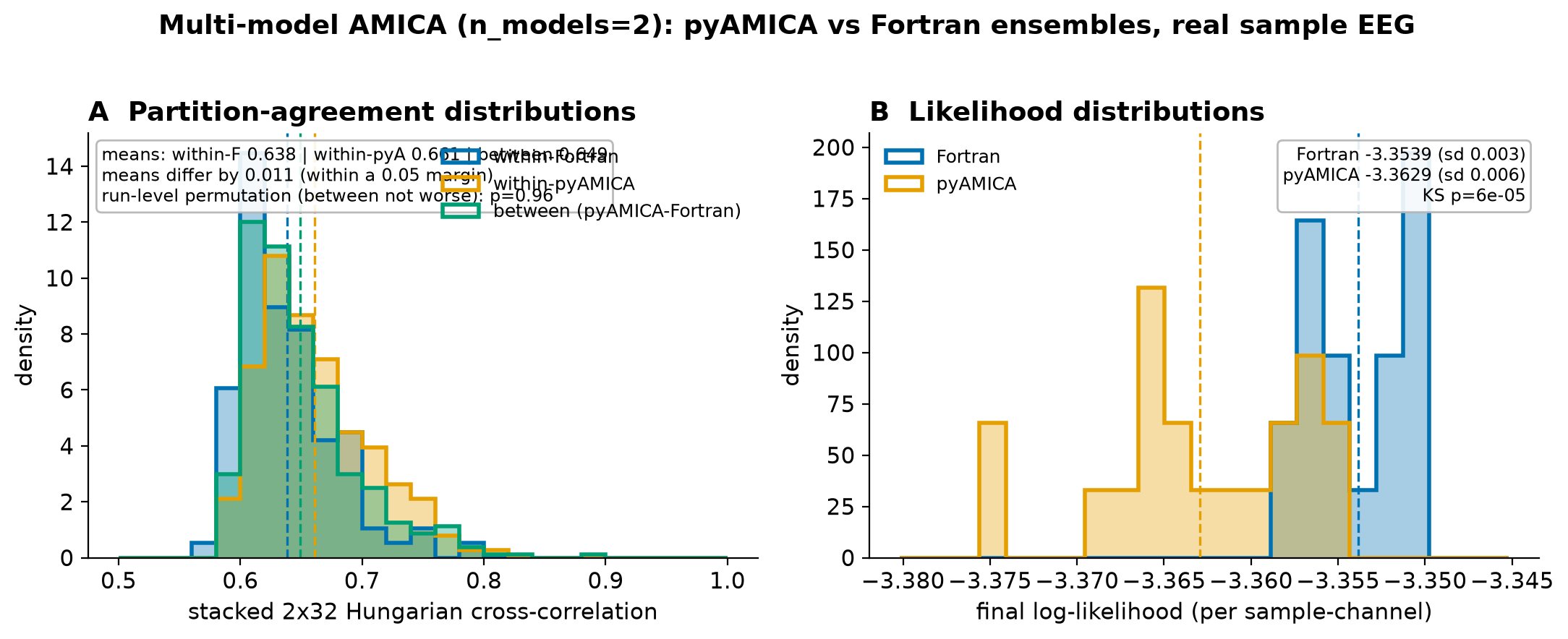
Pairwise Hungarian-matched component correlation for 20 pyAMICA and 20 Fortran multi-model fits of the sample EEG. The within-Fortran, within-pyAMICA, and between-implementation distributions overlap: the estimators sample the same solution space.

The three distribution means lie within 0.011 of each other (between 0.649, within-Fortran 0.638), well inside a \(\pm 0.05\) margin. To test this at the correct unit of analysis, we use a run-level permutation test: the 190/400 pairwise correlations are not independent (each of the 40 runs appears in ~39 pairs), so a Mann-Whitney or TOST applied to the pairwise values is pseudoreplicated and its p-value is invalid. Permuting the 40 runs as intact units instead (20000 permutations, statistic = within-Fortran minus between-implementation mean correlation) respects that dependence and finds no evidence that cross-implementation agreement is worse than Fortran's own run-to-run agreement (\(p = 0.96\)).

The single-run cross-correlation of ~0.65 is therefore intrinsic estimator spread, not a shortfall: Fortran agrees with itself at 0.64. The per-block sufficient statistics and one M-step are bit-exact against Fortran (~\(10^{-15}\)), so the update equations are correct; a small residual in the log-likelihood distribution (pyAMICA \(-3.363 \pm 0.006\) vs Fortran \(-3.354 \pm 0.003\); Kolmogorov-Smirnov \(p \approx 6\times10^{-5}\)) is an optimizer-quality effect, not a model-correctness defect (pyAMICA reaches Fortran's mean with about twice as many iterations).

Amari distance: a second, assignment-free metric

The correlation above needs a Hungarian assignment step to resolve component permutation before it can be computed. The Amari distance does not: it is permutation- and scale-invariant by construction, so it is a genuinely independent check on the same 20-run ensembles (.context/issue-27/ensemble.npz; recomputed by .context/issue-27/amari_distance.py with no re-fitting, since the raw unmixing matrices from the original 40 fits are already saved). Each stacked 2-model matrix is split into its per-model 32x32 blocks; since which Fortran model corresponds to which pyAMICA model is not identified, both label pairings are tried and the lower-distance pairing is kept, per run pair. This pairing correction is not free: on this ensemble it lowers the reported distance by ~0.02-0.03 versus always keeping the naive (unswapped) pairing, a similar order of magnitude to the within-Fortran/within-pyAMICA gap below, so part of that gap plausibly reflects how often each group happens to need the swap, not just genuine agreement differences.

Distribution (Amari distance, lower is better)	Mean	SD
within-Fortran (Fortran vs Fortran)	0.174	0.023
within-pyAMICA (pyAMICA vs pyAMICA)	0.154	0.019
between (pyAMICA vs Fortran)	0.163	0.022

The same run-level permutation test (20000 permutations, intact 40-run units) finds no evidence that between-implementation agreement is worse than Fortran's own run-to-run agreement (\(p > 0.999\)), agreeing with the correlation-based conclusion above.

Per-run detail (all 40 runs, both metrics)

Table 1 in the paper and the group summaries above report distribution means; the table below gives each of the 40 runs' own mean agreement to its own group's other 19 runs (within) and to all 20 opposite-implementation runs (between), for both metrics. Regenerate with uv run python .context/issue-27/amari_distance.py, which writes .context/issue-27/per_run_detail.csv.

implementation	run	corr within	corr between	Amari within	Amari between
Fortran	0	0.6164	0.6274	0.1880	0.1745
Fortran	1	0.6292	0.6568	0.1784	0.1592
Fortran	2	0.6465	0.6396	0.1694	0.1654
Fortran	3	0.6593	0.6740	0.1627	0.1508
Fortran	4	0.6323	0.6522	0.1797	0.1629
Fortran	5	0.6692	0.6773	0.1590	0.1488
Fortran	6	0.6660	0.6808	0.1628	0.1502
Fortran	7	0.6341	0.6400	0.1786	0.1678
Fortran	8	0.6285	0.6491	0.1779	0.1663
Fortran	9	0.6212	0.6341	0.1835	0.1702
Fortran	10	0.6308	0.6414	0.1794	0.1663
Fortran	11	0.6297	0.6444	0.1736	0.1614
Fortran	12	0.6334	0.6416	0.1782	0.1690
Fortran	13	0.6513	0.6630	0.1693	0.1574
Fortran	14	0.6666	0.6689	0.1584	0.1540
Fortran	15	0.6231	0.6254	0.1827	0.1750
Fortran	16	0.6147	0.6258	0.1903	0.1755
Fortran	17	0.6280	0.6483	0.1749	0.1632
Fortran	18	0.6441	0.6371	0.1691	0.1665
Fortran	19	0.6389	0.6505	0.1733	0.1637
pyAMICA	0	0.6317	0.6149	0.1690	0.1806
pyAMICA	1	0.6935	0.6777	0.1440	0.1529
pyAMICA	2	0.6624	0.6583	0.1545	0.1606
pyAMICA	3	0.6406	0.6459	0.1527	0.1561
pyAMICA	4	0.6493	0.6384	0.1506	0.1569
pyAMICA	5	0.6755	0.6591	0.1548	0.1622
pyAMICA	6	0.6339	0.6236	0.1677	0.1807
pyAMICA	7	0.6809	0.6788	0.1417	0.1479
pyAMICA	8	0.6780	0.6552	0.1508	0.1631
pyAMICA	9	0.6270	0.6206	0.1703	0.1823
pyAMICA	10	0.6855	0.6665	0.1474	0.1612
pyAMICA	11	0.6739	0.6556	0.1506	0.1612
pyAMICA	12	0.6321	0.6190	0.1617	0.1753
pyAMICA	13	0.6639	0.6610	0.1519	0.1597
pyAMICA	14	0.6866	0.6849	0.1460	0.1520
pyAMICA	15	0.6944	0.6672	0.1417	0.1559
pyAMICA	16	0.6576	0.6533	0.1551	0.1633
pyAMICA	17	0.6435	0.6249	0.1615	0.1756
pyAMICA	18	0.6753	0.6547	0.1442	0.1549
pyAMICA	19	0.6302	0.6180	0.1562	0.1655

Cross-platform device and precision invariance

The strongest reassurance that pyAMICA is a single, well-defined implementation is that it recovers the same independent components no matter where or how it runs. Fitting the same real EEG (ds002718 sub-002, 147,000 frames, 70 channels, 2000 iterations) on every backend and Hungarian-matching the unmixing components across them:

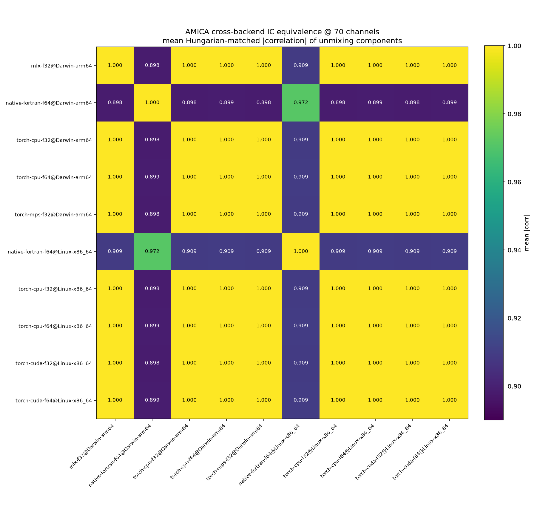
Mean Hungarian-matched |correlation| of the recovered components between every pair of backends. The eight torch/MLX combinations, CPU, CUDA, MPS, and MLX, at both float32 and float64, on macOS-arm64 and Linux-x86_64, all agree at 1.000.

Every torch/MLX backend is identical to every other at 1.000: the same decomposition on any device, at any precision, on either operating system. This is the definitive "float32 == float64" and "GPU == CPU" result. The two native-Fortran builds (macOS-arm64 and Linux-x86_64) agree with each other at 0.972 and with the torch/MLX cluster at ~0.90. That residual is not a backend defect: Fortran does not even reach 1.000 against itself across platforms, because each native run is seeded from the clock and settles into a different (equally valid) local optimum on the weakly-determined components only. As the decomposition becomes better-determined that gap closes (next section), and the component maps are visibly the same down every row:

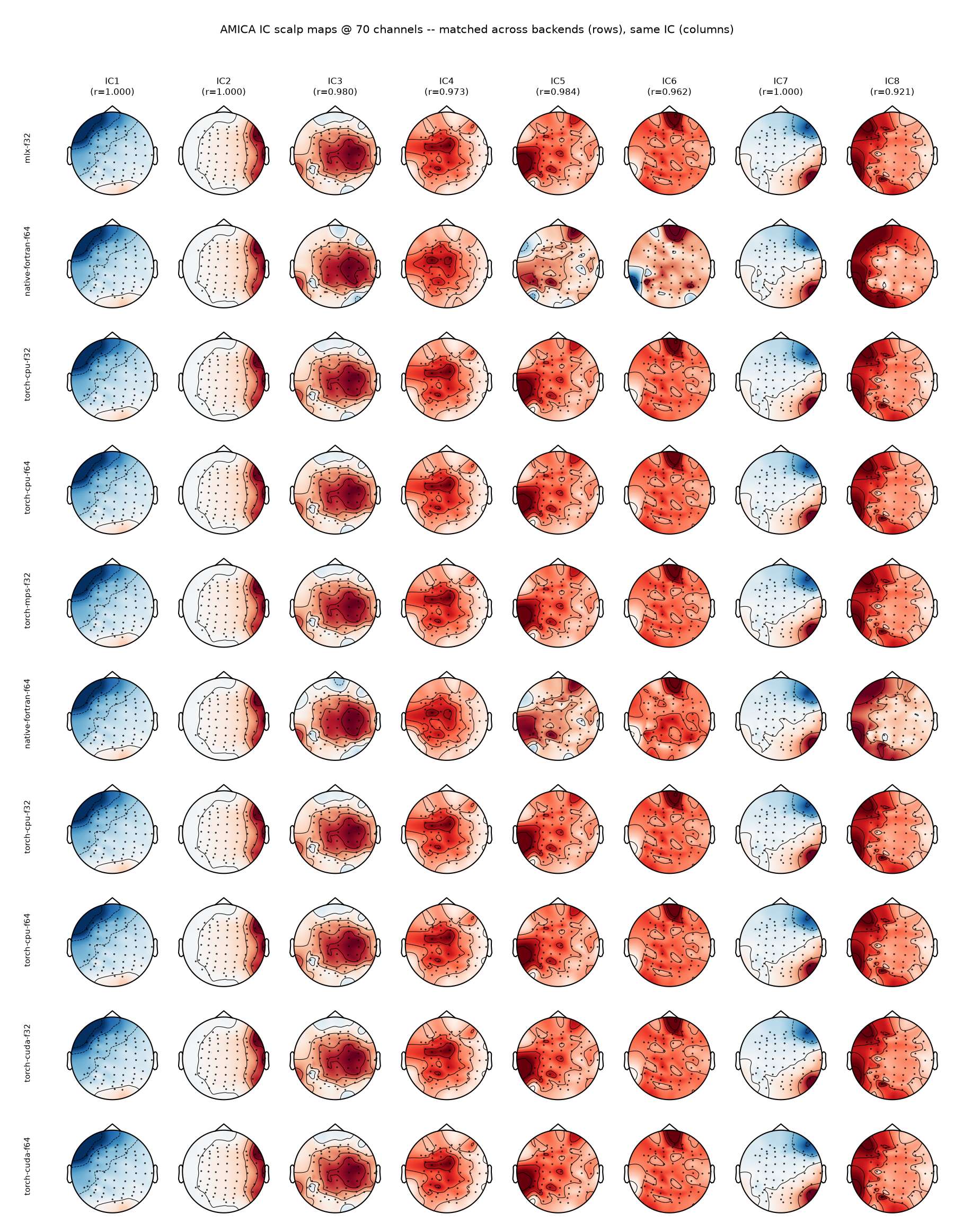
IC scalp maps at 70 channels, variance-ordered (IC1 = highest back-projected variance, EEGLAB convention), Hungarian-matched and sign-aligned across backends (rows). Each map is the de-sphered sensor-space projection. The well-determined components are indistinguishable across all backends.

Data adequacy and cross-backend equivalence

Whether backends recover the same components depends on how well-determined the decomposition is, captured by the data-adequacy factor:

\[k = \frac{\text{frames}}{\text{channels}^2}\]

As k grows, cross-backend component equivalence rises toward 1.0; at the rule-of-thumb minimum (k around 20-30) only the strongest components are backend-reproducible, while the rest are under-determined and settle into different but equally valid local optima (AMICA is non-convex). This is why the native-Fortran rows above sit at ~0.90 (70 channels, k = 30) rather than 1.0. Two independent sweeps confirm it.

Sweeping channels at fixed frames

Holding frames at 147,000 and increasing the channel count lowers k. Comparing MLX-float32 against the independent native-Fortran-float64 build (the hardest cross-implementation pair):

channels	k = frames/ch²	mean matched |corr|	components > 0.95
16	574	0.997	16/16
32	144	0.974	27/32
48	64	0.954	34/48
70	30	0.898	20/70

At high k every backend, including the independent Fortran build, recovers identical components (0.997, all 16/16 at k = 574). At k = 30, the rule-of-thumb minimum, only the strongest ~20/70 components are reproducible; the rest are under-determined.

Sweeping frames at fixed channels

Holding channels at 70 and increasing frames raises k, on the same real EEG:

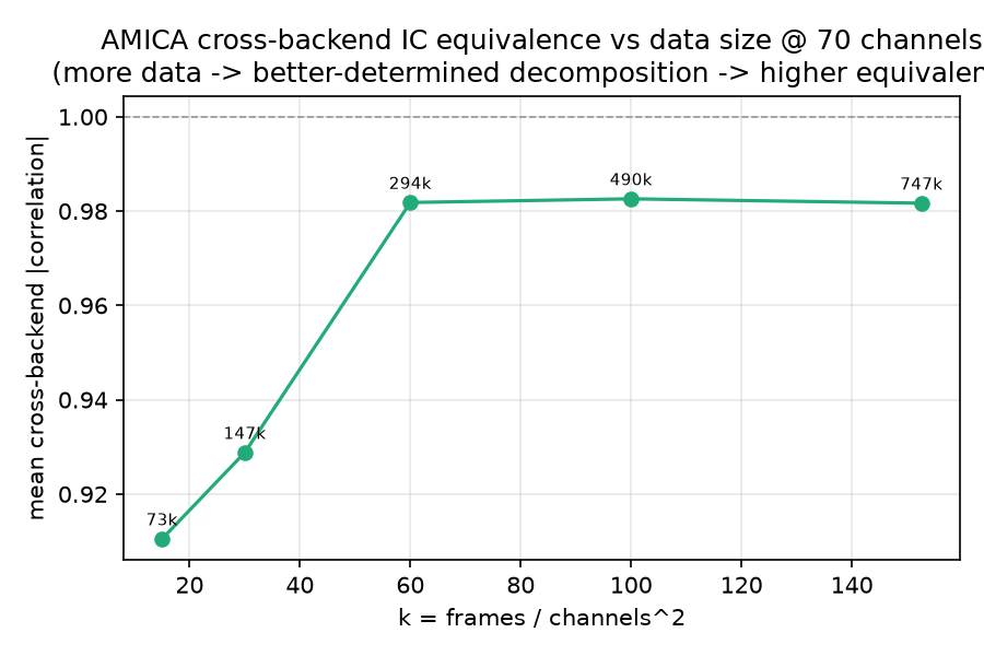
Mean Hungarian-matched cross-backend |correlation| versus \(k = \text{frames} / \text{channels}^2\) (70 channels, 2000 iterations, native-Fortran and PyTorch-CUDA float64/float32 backends). Equivalence saturates at ~0.98 once \(k \geq 60\).

frames	k	mean |corr|	components >0.95
73,500	15	0.911	55.2%
147,000	30	0.929	56.7%
294,000	60	0.982	90.0%
490,000	100	0.983	94.8%
747,750	152	0.982	92.4%

The k = 30 row here (0.929) sits above the 0.898 at k = 30 in the channel-sweep table because the two average different backend sets: the channel sweep reports only the hardest MLX-versus-native-Fortran pair, while this frame sweep averages over the native-Fortran and PyTorch-CUDA float64/float32 cluster.

The threshold is data-specific

For this recording the equivalence knee falls between k=30 and k=60; below it the backends settle into different (equally valid) local optima, above it they recover the same components. Where that knee sits depends on the data (signal-to-noise ratio, effective rank, source structure), so this is not a universal value of k. The plateau is ~0.98 rather than 1.0 because of intrinsic estimator spread and the float32 path, not a backend defect.

Why the plateau sits at ~0.98, not 1.0

At the largest data size (k=152) the residual below 1.0 splits cleanly by precision. The two double-precision implementations, an independent native Fortran binary and the PyTorch-CUDA backend, agree at 0.995:

Pair (at k=152)	|corr|
native-Fortran f64 vs PyTorch-CUDA f64	0.995
native-Fortran f64 vs PyTorch-CUDA f32	0.971
PyTorch-CUDA f64 vs PyTorch-CUDA f32	0.979

This is cross-implementation agreement, not just cross-device. The residual gap is dominated by the float32 path (rounding accumulated over 2000 iterations, plus an early stop when the natural-gradient learning rate hit its floor), which is a convergence/precision effect rather than a backend defect.

EEGLAB drop-in round-trip

pyAMICA writes the same on-disk format EEGLAB's AMICA plugin reads, so a fit is a drop-in replacement: no re-sorting, sign-flipping, or reformatting. After a fit, write_amica_output(dir) writes the raw binary files (gm, W, S, mean, c, alpha, mu, sbeta, rho, comp_list, LL) that EEGLAB's loadmodout15.m loads.

The round-trip is verified two ways:

• Byte-level: for a single model the written files are an exact float64 serialization of the fitted parameters. W and the symmetric zero-phase component analysis (ZCA) sphere are byte-identical in C order; the non-square mixture parameters and c/comp_list are column-major (Fortran layout), matching the reference amicaout files.
• Reader-level: the directory loads through loadmodout15.m (and its NumPy port loadmodout) with the expected shapes and the correct column-major layout. The MATLAB round-trip during development is what caught, and fixed, a column-major format bug in the mixture-parameter arrays.

variance_order() reproduces EEGLAB's IC ordering (IC1 = highest back-projected variance) in Python without a disk round-trip. For n_models > 1 the layout is self-consistent and round-trips through both readers, but is not byte-identical to a native multi-model run (see the multi-model discussion above). Full usage is in the EEGLAB interoperability guide; tests are in pyAMICA/tests/torch_tests/test_amica_ng_wrapper.py.

Performance across backends

Throughput on real EEG (OpenNeuro ds002718 sub-002; n_mix=3, pdftype=0, block_size=512, warmed, min-of-repeats). CPU, MPS, and MLX were measured on Apple Silicon; CUDA on a separate NVIDIA RTX 4090 host, so MLX-versus-CUDA reads as "best Apple-GPU path versus a strong NVIDIA GPU", not a same-box comparison.

Single-model, ms/iteration

channels	MLX f32	CUDA f32	CUDA f64	torch-CPU f32	torch-CPU f64	torch-MPS f32	NumPy f64
16	15.4	35.5	35.0	52	71	189	142
32	21.3	35.5	36.2	143	161	162	287
48	19.5	36.0	35.9	151	168	168	426
70	25.2	35.6	38.6	173	193	255	622

MLX is the fastest option on Apple Silicon and stays roughly flat with channel count (~7x over torch-CPU). PyTorch-MPS is not a win (at or worse than CPU), so use MLX rather than device="mps" on Apple hardware. CUDA float32 and float64 are near-identical here (launch-bound at this size). NumPy is the reference implementation, not a production path.

CPU core-scaling and native Fortran

The table above uses each platform's default thread count and has no Fortran row. A separate core-count sweep (--threads, real ds002718 sub-002 EEG, 70 channels, n_mix=3, pdftype=0, do_newton off, block_size=512) adds native Fortran (via OMP_NUM_THREADS) alongside torch-CPU (set_num_threads) and NumPy (threadpoolctl) on the same two machines as above, GPU backends run once since they are thread-independent:

backend (Intel Core i9-13900K / RTX 4090 workstation, 24 cores / 32 threads)	4c	8c	12c	16c	24c
native-fortran f64	69.5	43.2	49.0	40.0	30.0
torch-CPU f64	105.9	91.0	92.6	142.5	212.8
torch-CPU f32	84.6	69.5	71.8	70.9	73.0
NumPy f64	794.6	810.3	871.7	855.5	866.1

GPU (thread-independent, run once): CUDA f64 = 38.5, CUDA f32 = 36.2.

backend (Apple Silicon, 14 cores: 10P + 4E)	4c	8c
native-fortran f64	100.0	70.0
torch-CPU f64	131.4	169.9
torch-CPU f32	111.7	144.4
NumPy f64	627.0	627.4

GPU (thread-independent, run once): MLX f32 = 33.4, MPS f32 = 217.7.

Native Fortran with OpenMP is the only CPU backend that scales with cores: on all 24 of the 13900K's cores it beats the RTX 4090 (30 vs 38.5 ms/iteration), and on 8 of the Mac's 14 cores it is faster than either torch-CPU precision. torch-CPU f64 peaks around 8 cores then regresses from oversubscription (91 to 213 ms/iteration going from 8 to 24 cores on the workstation); torch-CPU f32 is faster and scale-stable but never catches the GPU. NumPy is thread-flat (BLAS/Python-bound) and slowest everywhere. MLX remains the efficiency winner overall: ~33 ms/iteration, flat, no tuning, beating a 450 W RTX 4090 and a 24-core Core i9-13900K workstation, at a fraction of the power and cost; native-Fortran@24c is marginally faster in raw ms/iteration only by pinning every core of a much larger, hotter machine. Native-Fortran timing at ≤32 channels is at or below the binary's ~10 ms stamp resolution, so trust the 48/70-channel scaling curve; the full 16/32/48/70-channel grid is in the result JSONs alongside .context/issue-84/phase2_cpu_scaling.md.

Multi-model (n_models=2), ms/iteration

channels	MLX f32	torch-CPU f32	torch-MPS f32	NumPy f64
32	38	187	291	869
70	45	224	270	928

The Apple-GPU win extends to multi-model: MLX ~38-45 ms/iteration, ~5x over torch-CPU, with MPS still losing.

Cross-backend log-likelihood agreement (single-model)

Every backend converges to the same log-likelihood to ~3 significant digits on real EEG, across device and precision, confirming the whole backend family end-to-end:

channels	MLX f32	CUDA f64	torch-CPU f64	torch-MPS f32	NumPy f64
32	-3.28634	-3.28635	-3.28636	-3.28635	-3.28620
48	-3.20951	-3.20952	-3.20953	-3.20951	-3.21019
70	-3.21579	-3.21562	-3.21560	-3.21570	-3.21315

Other validated behaviors

Beyond the core parity results, the following AMICA features are implemented and validated. Where the reference binary contains a bit-exact oracle it is used; where the reference code path is unrunnable (declared but never allocated, so it cannot be exercised even in Fortran) the feature is behavior-validated on real EEG instead, and guarded to a no-op so the parity results above stay byte-for-byte unchanged.

Behavior	Status	Validation
Best-iterate safeguard (keep_best, #51)	on by default	returns the highest-LL iterate; cuts multi-model LL sd from 12.7x to 2.0x Fortran's. Single-model parity stays bit-exact (monotone, no restore). ADR 0003
Per-model bias c update (#27)	on for n_models>1	Fortran update_c; per-block stats bit-exact; no-op for n_models=1
Component sharing (share_comps, #60)	off by default	Fortran identify_shared_comps ported; no bit-exact oracle (Spinv2 is unrunnable), behavior-validated; byte-identical when unshared
Outlier rejection (do_reject, #123)	off by default	good_idx mechanism in both backends; NumPy port validated vs the PyTorch backend
Degenerate-fit contract (#50)	always	a NaN or singular fit is refused (converged_ / stop_reason_); transform/get_*/save/write_amica_output raise instead of returning NaN sources

Tests live under pyAMICA/tests/: torch_tests/test_ng_backend.py, torch_tests/test_ng_sharing.py, torch_tests/test_amica_ng_wrapper.py, and test_numpy_reject.py.

Reproducing these results

Everything on this page runs from the bundled sample data and the reference binary, with no external download:

uv run python validate_implementations.py     # single- and multi-model parity report
uv run pytest                                  # the full parity/behavior test suite

The multi-model ensemble and Amari detail regenerate from saved fits (no re-fitting) with uv run python .context/issue-27/amari_distance.py. The cross-platform benchmark and equivalence figures are produced by benchmarks/benchmark_decompose.py (and the sweep scripts alongside it); the underlying findings are in .context/issue-84/ and .context/issue-90/.