How AMICA works

AMICA fits its generative model by maximum likelihood: it searches for the unmixing matrices, biases, model weights, and source-density parameters that make the observed data most probable.

The objective

Given \(N\) samples \(\mathbf{x}(t)\), AMICA maximizes the total log-likelihood

\[ \mathcal{L} = \sum_{t=1}^{N} \log \sum_{h=1}^{H} \gamma_h\,|\det \mathbf{W}_h| \prod_{i=1}^{n} p_{hi}\!\big(y_{hi}(t)\big), \qquad y_{hi}(t) = \mathbf{w}_{hi}^{\top}\big(\mathbf{x}(t)-\mathbf{c}_h\big), \]

over all parameters \(\{\mathbf{W}_h, \mathbf{c}_h, \gamma_h, \alpha_{hij}, \mu_{hij}, \beta_{hij}, \rho_{hij}\}\). The \(|\det\mathbf{W}_h|\) term is what keeps the unmixing matrices from collapsing to zero.

The algorithm

Because the model has hidden assignments (which model, and which mixture component, generated each sample), it is fit with expectation-maximization (EM), wrapped in a preprocessing and update loop.

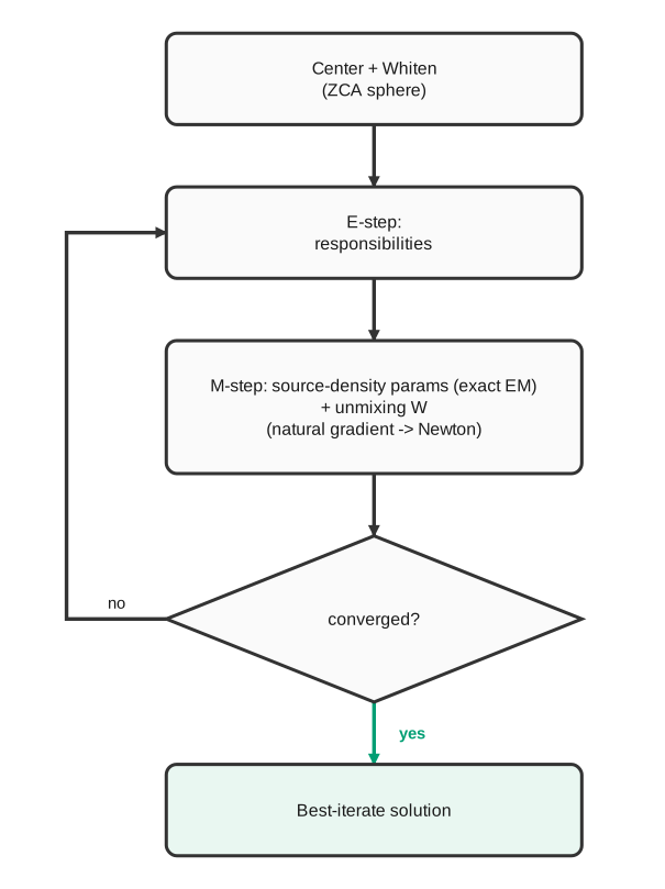
The AMICA fitting loop: preprocessing, then alternating E- and M-steps until the log-likelihood converges.

Preprocessing

The data are centered (mean removed) and whitened with a symmetric (ZCA) sphering matrix, matching the Fortran reference. Whitening removes second-order correlations so the iterations only have to resolve higher-order structure.

E-step (responsibilities)

Holding the parameters fixed, AMICA computes the posterior probabilities of the hidden assignments for each sample: the probability that model \(h\) generated it, and, within each source, the probability that mixture component \(j\) produced the activation. These responsibilities are the expected sufficient statistics used by the M-step.

M-step (parameter updates)

Holding the responsibilities fixed, AMICA updates the parameters:

• Source-density parameters (\(\alpha, \mu, \beta, \rho\)) are updated with the exact expectation-maximization closed-form expressions (a digamma equation for the shape \(\rho\)).
• Unmixing matrices are updated with the natural gradient, which accounts for the geometry of the space of matrices and converges far faster than the ordinary gradient:

\[ \Delta \mathbf{W}_h \;\propto\; \big(\mathbf{I} - \langle\, \mathbf{g}(\mathbf{y})\,\mathbf{y}^{\top}\rangle\big)\, \mathbf{W}_h, \]

where \(\langle\cdot\rangle\) is the responsibility-weighted average over samples and \(\mathbf{g}\) is the score function of the source density, \(g_i(y) = -\,\partial \log p_i(y)/\partial y\). For a single generalized Gaussian component this is \(g(y) = \rho\,\beta^{\rho}\,|y|^{\rho-1}\,\mathrm{sign}(y)\); for a mixture it is the responsibility-weighted combination of its components' scores. At the optimum the bracket vanishes, i.e. the sources are decorrelated from their own scores, a statement of independence.

• Newton update. Once the iterates are close, AMICA switches the unmixing update to a Newton step (using the per-source curvature of the likelihood), which sharpens convergence near the optimum. pyAMICA keeps this step positive-definite for stability.

Convergence and the returned solution

Each EM iteration increases the log-likelihood until it converges. Because the learning-rate schedule is not strictly monotone, pyAMICA returns the highest-likelihood iterate it visited (the best-iterate safeguard) rather than the last one, and reports its likelihood as final_ll_.

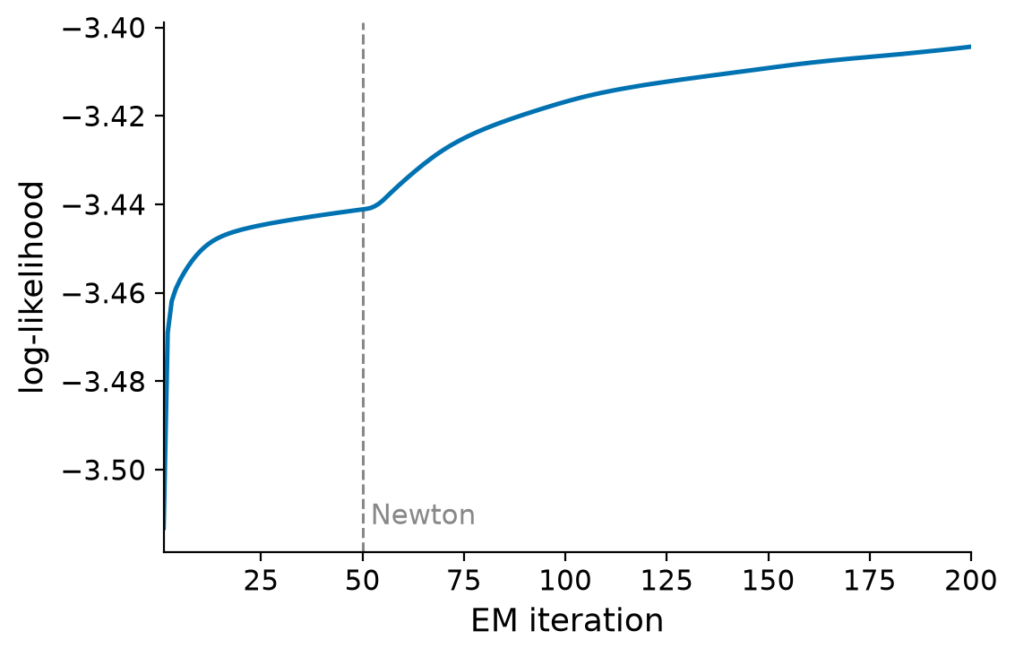
Log-likelihood versus iteration on the bundled sample EEG: the objective rises and converges toward the reference solution.

Relationship to the Fortran reference

Every M-step update in pyAMICA is derived to match the AMICA reference Fortran implementation, and on real sample EEG the natural-gradient backend reaches the same solution (log-likelihood and Hungarian-matched component correlation). See Validation & Parity for the acceptance criteria and how cross-backend equivalence depends on data adequacy.