What is ICA?

The cocktail-party problem

Imagine several people talking at once in a room, recorded by several microphones. Each microphone picks up a different mixture of all the voices. Independent Component Analysis (ICA) is the art of recovering the individual voices from the mixtures alone, without knowing who is speaking, where they stand, or how the room blends the sound. This is blind source separation: "blind" because we know neither the sources nor how they were mixed.

The same problem appears in electroencephalography (EEG). Each scalp electrode records a mixture of many overlapping brain and non-brain sources (cortical patches, eye blinks, muscle activity). ICA unmixes the electrode signals into maximally independent components, which often correspond to physiologically meaningful sources.

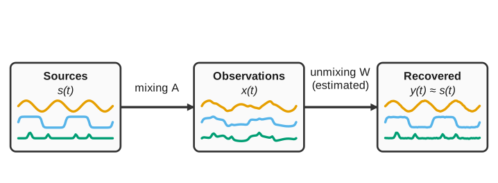
ICA recovers unknown independent sources from their observed linear mixtures by estimating an unmixing matrix.

The linear mixing model

ICA assumes the observations are an instantaneous linear mixture of the sources. With \(n\) sources and \(n\) sensors, at each time point \(t\):

\[ \mathbf{x}(t) = \mathbf{A}\,\mathbf{s}(t) \]

where

• \(\mathbf{s}(t) \in \mathbb{R}^{n}\) are the unknown, mutually independent source activations,
• \(\mathbf{A} \in \mathbb{R}^{n \times n}\) is the unknown mixing matrix (its columns are the sensor patterns, or "scalp maps," of each source),
• \(\mathbf{x}(t) \in \mathbb{R}^{n}\) are the observed sensor signals.

The goal is to estimate an unmixing matrix \(\mathbf{W}\) that inverts the mixing, so the recovered sources

\[ \mathbf{y}(t) = \mathbf{W}\,\mathbf{x}(t) \approx \mathbf{s}(t), \qquad \mathbf{W} \approx \mathbf{A}^{-1}, \]

are as close to the true sources as the data allow.

Why it works: independence and non-Gaussianity

Two assumptions make this well-posed:

1. Statistical independence. The sources are assumed mutually independent, so their joint density factorizes, \(p(\mathbf{s}) = \prod_i p_i(s_i)\). ICA looks for the \(\mathbf{W}\) that makes the outputs \(y_i\) as independent as possible.
2. Non-Gaussianity. By the central limit theorem, a sum of independent variables is "more Gaussian" than its parts, so a mixture looks more Gaussian than the underlying sources. Recovering the sources is therefore equivalent to finding the projections that are maximally non-Gaussian. A crucial corollary: Gaussian sources cannot be separated (a rotation of independent Gaussians is still independent Gaussians), so ICA requires at most one Gaussian source.

The geometry is easy to see with two sources. Independent sources fill an axis-aligned region; mixing shears and rotates that region; ICA finds the transform that restores the independent axes.

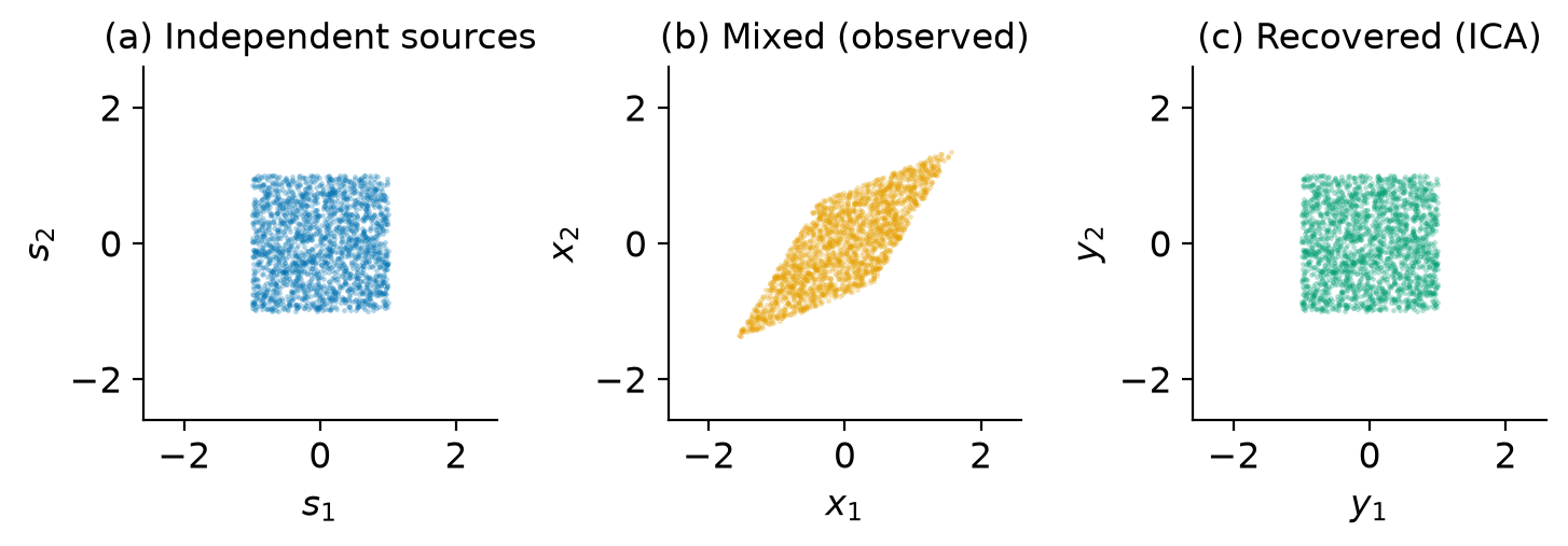
Left: two independent sources. Middle: the observed mixture is sheared and rotated. Right: ICA recovers the independent axes (up to order and scale).

Preprocessing: centering and whitening

In practice the data are first centered (mean removed) and whitened (also called sphering): linearly transformed so the channels are uncorrelated and have unit variance. Whitening removes all second-order structure, reducing the remaining ICA problem to finding an orthogonal rotation, which is both faster and better conditioned. pyAMICA uses a symmetric (ZCA) whitening that matches the Fortran reference.

What ICA cannot pin down

Because \(\mathbf{A}\) and \(\mathbf{s}\) are both unknown, two ambiguities are irreducible:

• Permutation. The sources can be recovered in any order.
• Scale and sign. Each source's amplitude (and sign) is arbitrary, since a scalar can move between a column of \(\mathbf{A}\) and the corresponding source.

These do not affect the usefulness of the components; they only mean component indices and scaling are conventions, not ground truth. pyAMICA follows the EEGLAB conventions for ordering and sign where it matters (see Validation & Parity).

Next: What is AMICA?, which relaxes the fixed-source-density assumption and adds multiple models.