What is AMICA?

Classical ICA algorithms assume a single, fixed shape for every source density (for example a logistic or Laplacian distribution). Real signals rarely oblige: some EEG sources are sharply peaked and heavy-tailed (super-Gaussian), others are flatter (sub-Gaussian), and the mixing regime itself can change over time. Assuming the wrong density biases the separation.

AMICA (Adaptive Mixture ICA) removes that limitation with two "adaptive mixture" ideas layered on top of ICA.

Idea 1: adaptive source densities

Instead of fixing the source distribution, AMICA models each source as a mixture of generalized Gaussians and learns its shape from the data.

The generalized Gaussian density with location \(\mu\), scale \(\beta\), and shape \(\rho\) is

\[ q(y;\rho,\mu,\beta) = \frac{\rho\,\beta}{2\,\Gamma(1/\rho)}\, \exp\!\big(-\beta^{\rho}\,|y-\mu|^{\rho}\big). \]

The shape parameter \(\rho\) controls the tails:

• \(\rho = 2\) recovers the Gaussian,
• \(\rho = 1\) is the Laplacian (peaky, super-Gaussian),
• \(\rho < 2\) is super-Gaussian (heavier-tailed, more kurtotic),
• \(\rho > 2\) is sub-Gaussian (flatter, platykurtic).

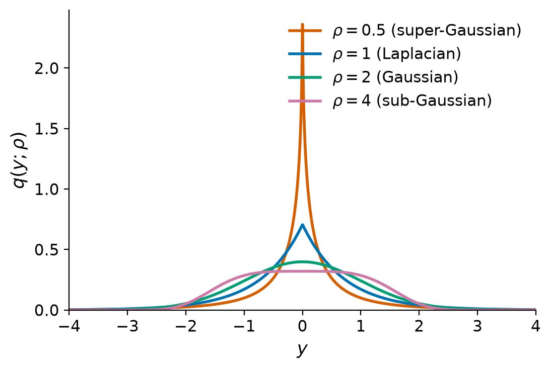
The generalized Gaussian family spans super-Gaussian (\(\rho<2\)), Gaussian (\(\rho=2\)), and sub-Gaussian (\(\rho>2\)) shapes with a single parameter.

Each source density is a weighted mixture of \(m\) such components, so it can take on skewed and multimodal shapes:

\[ p_i(y) = \sum_{j=1}^{m} \alpha_{ij}\, q\!\big(y;\rho_{ij},\mu_{ij},\beta_{ij}\big), \qquad \sum_{j=1}^{m}\alpha_{ij}=1 . \]

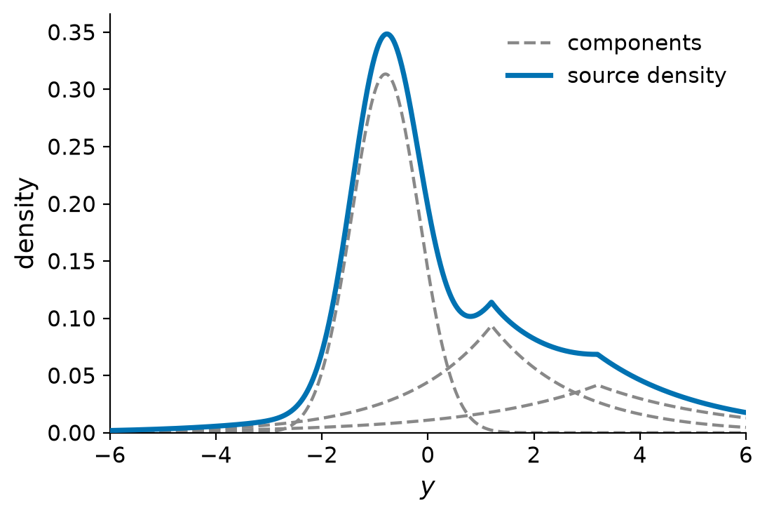
An adaptive source density (solid) as a weighted sum of generalized Gaussian mixture components (dashed).

pamica supports all five source-density families of the reference implementation (generalized Gaussian is the default), plus an extended-Infomax switcher that flips each source between super- and sub-Gaussian by the sign of its kurtosis. The legacy NumPy backend fits the generalized Gaussian only.

AMICA settles ICA's scale ambiguity (What ICA cannot pin down) by convention: each component's mixing vector is kept at unit norm, and the source's amplitude is carried by the locations \(\mu_{ij}\) and scales \(\beta_{ij}\) of its density. AMICA restores that convention after every update by rescaling each component (doscaling, on by default), an exact change of scale that leaves the likelihood unchanged (see How AMICA works).

Idea 2: multiple ICA models

A single unmixing matrix assumes one fixed mixing regime for the whole recording. AMICA instead fits a mixture of \(H\) ICA models, each with its own unmixing matrix \(\mathbf{W}_h\), bias \(\mathbf{c}_h\), and source densities. A per-sample responsibility softly assigns each time point to the model that explains it best, so AMICA can capture non-stationarity and distinct regimes in the data.

The full generative model gives each observation the mixture likelihood

\[ p(\mathbf{x}) = \sum_{h=1}^{H} \gamma_h\, |\det \mathbf{W}_h| \prod_{i=1}^{n} p_{hi}\!\big(\mathbf{w}_{hi}^{\top}(\mathbf{x}-\mathbf{c}_h)\big), \]

where \(\gamma_h\) are the model weights (\(\sum_h \gamma_h = 1\)), \(\mathbf{w}_{hi}^{\top}\) is the \(i\)-th row of \(\mathbf{W}_h\), and the \(|\det \mathbf{W}_h|\) (Jacobian) term accounts for the change of variables from \(\mathbf{x}\) to the sources.

With \(H = 1\) this reduces to ordinary ICA with adaptive source densities. That single-model case is the default, and it is where pamica's parity with the Fortran reference is established (see Validation & Parity).

AMICA also supports shared components across models (components whose scalp maps are nearly identical in two models are merged, so the models share one mixing vector and one density) and outlier rejection (samples whose likelihood is far below the rest are dropped from the fit). Both are off by default.

Next: How AMICA works, which fits this model by maximizing its likelihood.