How AMICA works

AMICA fits its generative model by maximum likelihood: it searches for the unmixing matrices, biases, model weights, and source-density parameters that make the observed data most probable.

The objective

Given \(N\) samples \(\mathbf{x}(t)\), AMICA maximizes the total log-likelihood

\[ \mathcal{L} = \sum_{t=1}^{N} \log \sum_{h=1}^{H} \gamma_h\,|\det \mathbf{W}_h| \prod_{i=1}^{n} p_{hi}\!\big(y_{hi}(t)\big), \qquad y_{hi}(t) = \mathbf{w}_{hi}^{\top}\big(\mathbf{x}(t)-\mathbf{c}_h\big), \]

over all parameters \(\{\mathbf{W}_h, \mathbf{c}_h, \gamma_h, \alpha_{hij}, \mu_{hij}, \beta_{hij}, \rho_{hij}\}\). The \(|\det\mathbf{W}_h|\) term is what keeps the unmixing matrices from collapsing to zero.

The algorithm

Because the model has hidden assignments (which model, and which mixture component, generated each sample), it is fit with expectation-maximization (EM): a preprocessing step, then a loop of iterations. Each iteration runs in the same order as the Fortran reference: the E-step, then the checks, then either an exit or the parameter update.

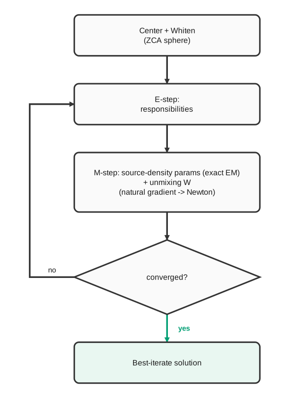
The AMICA fitting loop: preprocessing, then iterations of E-step, checks and update, until a stopping check fires or the iteration budget runs out.

Preprocessing

The data are centered (mean removed) and whitened with a symmetric zero-phase component analysis (ZCA) sphering matrix, matching the Fortran reference. Whitening removes second-order correlations so the iterations only have to resolve higher-order structure. When the data are rank-deficient, or a principal component analysis (PCA) reduction is requested with pcakeep, the sphering also reduces the data to the dimensions that are kept, and the model has that many sources.

1. E-step

Holding the parameters fixed, AMICA computes the posterior probabilities of the hidden assignments for each sample: the probability that model \(h\) generated it, and, within each source, the probability that mixture component \(j\) produced the activation. These responsibilities are the expected sufficient statistics the update needs. The same pass over the data gives the log-likelihood of the current parameters and the direction in which the unmixing matrices should move, together with its size, the gradient norm.

2. Checks

Before anything is updated, the iteration looks at what the E-step found.

• A log-likelihood decrease. The update steps do not guarantee that the likelihood rises: a step can overshoot. When the likelihood falls from one iteration to the next, AMICA halves the learning rate of the unmixing update (by lratefact), so this iteration's step is already the smaller one. Every maxdecs decreases it also lowers the ceiling the learning rate can climb back to, so the rate cannot keep returning to the value that overshot.
• Stopping checks. The fit stops when the likelihood has risen by less than min_dll for more than maxincs iterations in a row, when the gradient norm falls to min_nd, or when a decrease finds the learning rate already at its floor (minlrate). A non-finite log-likelihood or update direction also ends the fit, and marks it degenerate: every output method then refuses the model, so no NaN sources reach an analysis.

The likelihood and gradient checks cannot fire on the first iteration, which has no earlier likelihood to compare with.

3. Exit, or update

If a check fired, the fit leaves here, before any parameter moves, so the parameters it returns are the ones whose likelihood it has just computed. Otherwise the M-step updates the parameters, with the learning rates the checks have just set:

• Model weights, biases and mixture weights (\(\gamma_h\), \(\mathbf{c}_h\), \(\alpha\)) take their exact expectation-maximization values, closed-form functions of the responsibilities.
• Unmixing matrices move by the natural gradient, which accounts for the geometry of the space of matrices and converges far faster than the ordinary gradient:

\[ \Delta \mathbf{W}_h \;\propto\; \big(\mathbf{I} - \langle\, \mathbf{g}(\mathbf{y})\,\mathbf{y}^{\top}\rangle\big)\, \mathbf{W}_h, \]

where \(\langle\cdot\rangle\) is the responsibility-weighted average over samples and \(\mathbf{g}\) is the score function of the source density, \(g_i(y) = -\,\partial \log p_i(y)/\partial y\). For a single generalized Gaussian component this is \(g(y) = \rho\,\beta^{\rho}\,|y|^{\rho-1}\,\mathrm{sign}(y)\); for a mixture it is the responsibility-weighted combination of its components' scores. At the optimum the bracket vanishes, that is, the sources are decorrelated from their own scores, a statement of independence. The step is scaled by the learning rate, which climbs back toward its ceiling a little on every update.

• Newton step. With Newton enabled, from iteration newt_start on, AMICA replaces the natural-gradient direction with a Newton step, which uses the per-source curvature of the likelihood and converges faster near the optimum. An iteration whose curvature is not positive definite falls back to the natural gradient, which keeps the step stable. Newton is off by default, as in the reference binary's compiled default; pass do_newton=True to turn it on, as the reference's bundled input.param does.
• A-freeze windows. From iteration share_start on, AMICA holds the unmixing update, and its learning-rate climb, on the six iterations that start at each multiple of share_iter: with the defaults (share_start = share_iter = 100), on iterations 100-105, 200-205, and so on. The windows give the models time to settle after component sharing merges components, but the reference applies them to every fit, with or without sharing, and so does pamica. The other parameters keep updating during a window.
• Source-density parameters (\(\mu, \beta, \rho\)) take their exact expectation-maximization values: closed-form expressions for the locations and scales, and a digamma equation for the shape \(\rho\), stepped by its own learning rate.
• Rescaling (doscaling). ICA cannot tell a large source with a narrow density from a small source with a wide one. After the update, AMICA divides each component's mixing vector by its norm and rescales that component's density location and scale to match. This is an exact change of scale: the log-likelihood does not change, and every component's mixing vector has unit norm.

An update that leaves any parameter non-finite ends the fit at once, also marked degenerate. After the update come the optional steps: the extended-Infomax switch between super- and sub-Gaussian densities (pdftype=1), the component-sharing scan (share_comps), and outlier rejection (do_reject). Then the next iteration starts with its E-step.

Convergence and the returned solution

The log-likelihood rises over a fit, but not at every iteration: a step can overshoot, which is what the decrease response corrects. A fit ends on a stopping check or when it reaches max_iter. After a stopping check, the returned parameters are exactly those whose likelihood was last computed. At max_iter the last iteration still takes its update, as in the reference, so the last likelihood computed belongs to the parameters one update earlier.

Because the learning-rate schedule is not monotone, pamica by default returns the highest-likelihood iterate it visited (the best-iterate safeguard, keep_best), which is the last one unless the fit ended below an earlier peak, and reports its likelihood as final_ll_. The reference has no such safeguard, and pamica turns it off under component sharing and outlier rejection, where likelihoods from different iterations are not comparable.

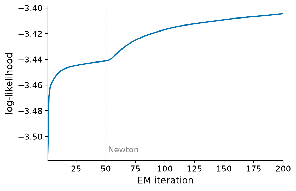
Log-likelihood versus iteration on the bundled sample EEG: the objective rises and converges toward the reference solution.

Relationship to the Fortran reference

Every step above follows the AMICA reference Fortran implementation (amica15), in the same order within each iteration, and on real sample EEG the natural-gradient backend reaches the same solution (log-likelihood and Hungarian-matched component correlation). See Validation & Parity for the acceptance criteria and how cross-backend equivalence depends on data adequacy, and pamica vs. AMICA for every place pamica deliberately differs.